Previous Assignments
- Author:
Prof. dr.ir. T.N.Olsthoorn
Assignment Jan 2022. Wells along a river.
Problem statement
Consider a region to the right of a straight river which is in direct contact with a water table aquifer that has a transmissivity of \(kD=900\,\mathrm{m^{2}/d}\) or an average saturated thickness of \(D=30\,\mathrm{m}\) and a horizontal conductivity of \(k=30\,\mathrm{m/d}\). The specific yield of the aquifer is \(S_{y}=10%\ensuremath{\%}\).
There is regional groundwater flow directed towards that river at a rate of \(q=0\,\mathrm{m^{2}/d}\).
A groundwater pumping station with one well is installed at \(L=1500\,\mathrm{m}\) distance from the river which starts extracting at time \(t=0\) at a rate of \(Q=1200\,\mathrm{m^{3}/d}\). For the analysis the aquifer thickness can be considered constant as given above.
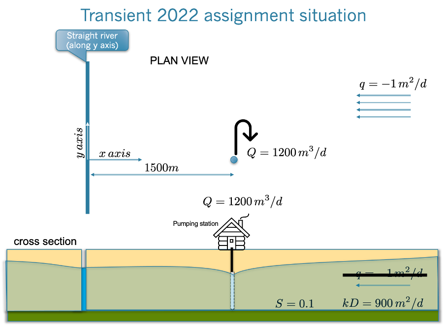
Fig. 48 Situation, map and cross section.
Make a picture of the water table at a line through the pumping well perpendicular to the river at t the following times 0.001, 1day, 1 week, 1 month, 1 year, 10 years after the start of the extraction.
Make a picture of the head contours in top view after 1 month, 1 year and 10 years.
Make a picture of the flow direction in top view after 1 month, 1 year and 10years.
Show the inflow from the river
The river stage varies like a sine with an amplitude of 2 m and a cycle time of 1 year. How far from the river can this fluctuation be felt if one takes 10 cm amplitude as a criterion?
Plot the envelopes on top of the steady state (or the head after years of constant pumping).
How much is the delay of the stage wave in the river at the point where the amplitude is still only 10 cm?
There is a sudden shower of rain equal to 240 mm, which raises the water table suddenly and uniformly. By how much will the water table rise due to this sudden recharge if it is assumed that all this precipitation will add to the groundwater?
Show the development of the water table over time (for a few times after the shower took place) by adding its effect to the steady-state situation (pumping station has been pumping continuously for at least 10 years?
How to work out the assignment
Work out these questions using Jupyter notebooks in Python. For that download Anaconda python from the Anaconda website.
We’ll introduce this in the course and will practice examples also in the course.
To become familiar google for “Mark Bakker exploratory computing with Python”. There you’ll find an introduction and a set of notebooks to exercise as do the 2nd year students at the TUDelft. These tutorials are really very good.
I expect the assignment notebook result two days after the written exam. The reason is that the mark for the assignment is 30% and that of the written exam makes up 70% of the result, so I need both when I score the exams.
Assignment Jan 2021. Wells along a river in a closed valley.
A groundwater extraction station with three wells is to be realized in a very long, \(L=5\,\mathrm{km}\) wide, almost straight valley. The valley is bounded by bedrock while the sediments below the water table can be considered \(D=50\,\mathrm{m}\) thick, layer of sand on top of pratically impervious material. As shown in the cross section of Figure 1, a river, that may be considered fully penetrating and in direct contact with the aquifer, flows along one of the valley walls. The water table is 5 m below ground surface at the center line of the valley, where the wells are to be installed. As is shown on the map in Figure 2, the three wells will be placed 500 m apart along the center line of the valley. Each well will pump \(Q=2400\,\mathrm{m^{3}/d}\).
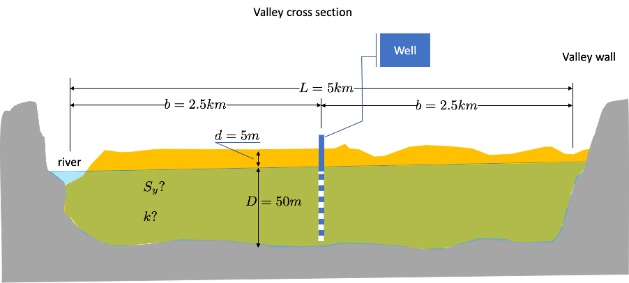
Fig. 49 Cross section through the valley.
One pumping well and three observation wells were installed first, and a pumping test was done on it to determine the aquifer properties, i.e. its transmissivity \(kD\) and its storage coefficient, i.e. its specific yield \(S_{y}\). The pumping lasted for 1 months (30 days) at a rate of \(Q=600\,\mathrm{m^{3}/d}\). During this time, the heads in the well and in the piezometers were monitored from which the drawdown relative to the initial situation was determined. These darwdowns are provided in a table in an accompanying spreadsheet. The header of the table shows at which distance from this well the observation wells were placed. These observation wells (also called piezometers) are not shown on the cross section and the map because they are too close to the well to be shown on this scale.
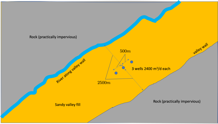
Fig. 50 Map of the valley with the final three well in place. The observation wells used in the pumping test are not shown as they are too close to the well for the scale of this map.
Each student obtains a spreadsheet with unique the pumping-test data. You find the spreadsheet with your name in the folder on BBB named “Assignment”.
Each student obtains a spreadsheet with unique the pumping-test data. You find the spreadsheet with your name in the folder on BBB named “Assignment”.
Assignment questions
With the drawdown data given in the accompanying spreadsheet, determine the aquifer properties kD and Sy.
How far out into the aquifer does the drawdown during the pumping test reach?
Is there during the pumping test an influence from the river and or the valley wall on the drawdowns?
What will be the development of the drawdown in the final 3 wells assuming they are fully penetrating and are not clogged?
Show the development of the drawdown along a line perpendicular to the valley axis through the center well.
Show the development of the drawdown along the valley axes through the 3 wells.
Show the development of the inflow from the river into the aquifer due to the three wells.
Show the drawdown in a map after it has become steady srate.
What is the required depth of the pumps, given that the wells have an extra drawdown due to partial penetration and clogging which doubles the drawdown relative to the case of unclogged fully penetrating well and given that the top of the pump has to be at least 1.5 m below the water table in the well.
Tip: Set the computation up for a single arbitrary point first not worrying about superposition the results for many points (like along a line or in a map) and not worrying about superposition across the river and the valley wall. This can all be included step by step.
The pumping-test data
TODO: Filled in here.
Assignment Jan 2020. Same as Jan 2018
Essentially the same assignment as in 2018 was used in 2020.
Assignment Jan 2019. A building pit next to a river.
Problem statement
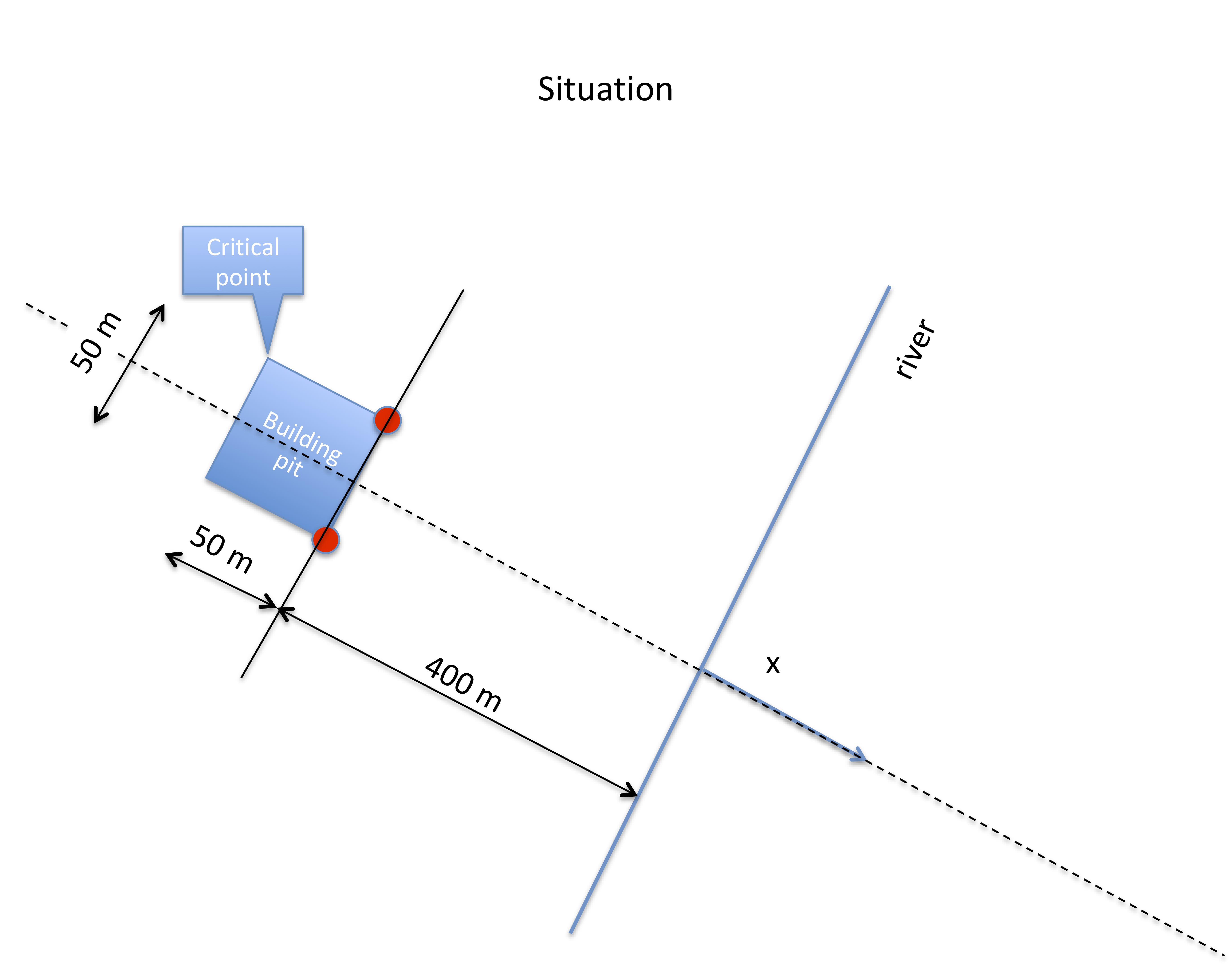
Fig. 51 Situation sketch.
A large construction is to be realized next to a river that is in direct contact with the aquifer next to it. The building pit measures 50x50 m and river side is at 400 m distance from the river shore.
Transmissivity and storage coefficient are given: \(kD=900\,\mathrm{m^{2}/d}\), \(S_{y}=0.25\).
The drawdown everywhere in the building pit must be at least 5 m, to be reached within one month of pumping.
The pumping will continue after this month for 5 more months during which the drawdown is to be maintained. However the pumping can be reduced after the first month. Adjust the pumping once per month, such that at the end of each month the darwdown fullfils the requied 5 m.
After 6 months, pumping is stopped, so that the water levels can restore.
Questions
On which two corners of the builing pit should you place the two extraction wells to have most effect?
Find the most critical point and make sure that the drawdown is as required at that point.
Show the extraction as a function of time from the start until one year after the stop. Also plot the drawdown at the critical location for this period.
Compute as a function of time the flow from the river into the groundwater system. It is assumed that the groundwater head is initially uniform and equal to the river stage (water level in the river). Do this for the averate flow during the 6 month of building pit operation (ignore the variation in the extraction for simplicity).
How much time is required after stopping until about 90% of the drawdown has disappeared?
After exactly 3 months, the water level in the river rises suddenly by 1 m and stays so during one month, after which it suddenly returns to its original level.
To what extent does this wave affect the water level in the building pit if no measure is taken?
What must be the extraction during this month to guarantee that the building pit fulfills the required 5 m drawdown relative to the original water level? If both effects do not overlap, say so, and explain what you could to as building-pit owner to better counteract the effect of the wave in the river stage on the head below the building pit
If the river is influenced by sea tide, such that its level fluctuates twice a day between +1 and -1 m relative to the average value. How does this tide influence the required pumping? Is the location of the most critical point still the same?
How much is the delay between the tide in the river and the fluctuation at the critical point in the building pit?
Hints
Work out the assigment in this Jupyter notebook. Take some time to become familiar with it. There is a tremendous amount of help on the internet to get you going. The site on ‘github.com/Olsthoorn/TransientGroundwaterFlow‘ hold numerous examples from the syllabus in the form of ‘jupyter notebooks‘.
Also refer to the notebooks for the second year students of the TUDelft by Mark bakker (search for ‘Bakker exploratory‘ computing to find them).
You will gain some experience with the Notebooks (see their help)
with python
with numpy
with functions in scipy
Make sure your assigment is a self-contained document, that you could also export as html or pdf for sharing to those who do not have python installed.
Assignment Jan 2018. Water company uses ASR system to prevent river inflow during summer.
The assignment is essentially the same as the one of 2017.
Assignment Jan 2017. Water company uses ASR system to prevent extraction from tiver during summer
Problem statement
A water company extracts water from a small river to treat and distribute it as drinking water for the population of a small town nearby. This is not a problem in winter. However, due to growing demand for drinking water and growing environmental concern, extraction has become more and more problematic during summers when the discharge of this small river is at its lowest. The environmental agency has recently even forbidden to further extract water from the river during the summer months.
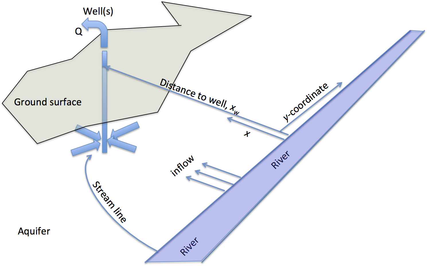
Fig. 52 Situation sketch.
In order to solve the problem that this causes for the drinking water supply, the drinking water company has suggested an Aquifer Storage and Recovery system (these so-called ASR systems are becoming more and more popular). It wants to take in more river water during winter and inject it through a well (or wells) at some distance from the river into the local water-table aquifer, so that this water can be extracted during the next summer. This way, no water-intake will be necessary during the summer months.
However, the debate that took off between the water company and the environmental agency focuses on whether, or to what extent, this ASR system really makes sense. Can you really store the water in winter and extract it during summer without substantially affecting the already low summer-discharge of the river? Will not much of the stored water flow back to the river through the aquifer during winter? And would the extraction not induce an infiltration from the river into the aquifer during summer, so that there is still a water intake, the only differece now being that it will be invisible?
It’s your task as hydrologist of the environmental agency to answer this question and illustrate it quantitatively and also explain it clearly. Your explanation should include why and how you derived your answer. It should show the math and the code.
It is obvious that ASR will work if the distance between the well and the river is large enough. But how large is large enough, and on what does it depend? The water company suggested a distance of 500 m from the river. Should the environmental agency agree?
Hints and further information:
To analyse this system, at least coarsely, simplify the injection and extraction regime and apply superposition. Superposition allows to only consider the well and treat the river as a fixed-head boundary using a mirror well. Simplify the river to a straight line along the y-axis and place the well at distance \(x_{w}\) from this line at coordinate \((x_{w},0)\). That is, the x-axis is perpendicular to the river.
The drinking water demand, \(Q\), is considered constant year-round at \(150\,\mathrm{L/d}\) per inhabitant for the 10000 inhabitants of the town.
Assume the following injection and recovery regime:
The water company well extracts during 3 summer months (June, July, Aug) its full demand
It compensates that during 6 winter months (October-March) by injecting half its daily capacity.
There is neither injection nor extraction during the months April, May and September.
The idea is to analyse this ASR system by computing the exchange between the aquifer and the river due to the well.
When you have coded the problem for this particular distance of 500 m, experiment with this distance to come up with a distance that realy makes sense in terms of not inducing loss of river water during the summer months. That is, try 1000 and 2000 m.
Use \(kD=900\,\mathrm{m^{2}/d}\), \(S_{y}=0.2\).
Steps to take:
Use Theis’ well function to compute drawdowns:
\[s(t,t)=\frac{Q}{4\pi kD}\mathrm{W}(u)\mbox{, with }\mathrm{W}(u)=-scipy.special.expi(-u)\mbox{ and }u=\frac{r^{2}S}{4kDt}\]- From Theis’ well function\[\mathrm{W}(u)=\intop_{u}^{\infty}\frac{e^{-y}}{y}dy\]
derive the flow \(Q(r,t)\,\mathrm{[L^{3}/T]}\) and the specific discharge \(q(r,t)\,\mathrm{[L^{2}/T]}\) in the aquifer at distance \(r\) from the well.
To simulate the river, apply a mirror well.
Compute the exchange between aquifer and river, derive the specific discharge \(q\,\mathrm{[L^{2}/T]}\) perpendicular to the river at an arbitrary point \(y\).
Compute this specific discharge for a large number of points between \(-ax_{w}<y<ax_{w}\), where \(a\) is sufficiently large, thus covering a large enough track of the river to capture about the full induced exchange between aquifer and the river. See below how appropriate \(y\)-coordinates can be generated in Python.
Numerically integrate this specific discharge along the river to obtain the total exchange between river and aquifer. (Numerical integration is easy when uing the Simpson’s trampezium rule).
Having the code to do this for a single time, it can readily be extended for a large number of times.
Check that for large times, the total flow between aquifer and river should be about the total discharge of the well if the well is continuously injecting.
Finally simulate the actual flow regime with 6 month injection and 3 months extraction as explained above. Simulate for a period of 5 years. This simulation requires superposition in time.
Appropriate \(y\)-coordinates may be generated in Python as follows:
y = np.hstack(( -np.logspace(0, np.log10(a * xw), Np)[::-1], np.logspace(0, np.log10(a * xw), Np))
Where \(a\) may be taken 10 and the number of points, \(N_{p}\), can be taken 500 for example.
Suggestions
It is probably easiest to analyze everything in time units of months instead of days, 5 years time then runs from 0 to 60 months.
Learn to define and use functions in Python to keep overview and prevent repeating code.
If you consider this too complicated, then anlyse at least the situation for only the river point closest to the well.
Start by plotting the head.
When this works focus on the discharge.
Don’t hesitate to ask questions and for help.
The data as a csv (comma separated values)
You can select the values below and copy-paste them in a text file to be read by python (use the pandas module for convenience for working with tables and reading them including excel sheets and csv files.)
date,n,month,year,Qfac,Q,dQ,tch
2010-01-01,1,1,2010,0.5,750,750,0
2010-02-01,2,2,2010,0.5,750,0,31
2010-03-01,3,3,2010,0.5,750,0,59
2010-04-01,4,4,2010,0,0,-750,90
2010-05-01,5,5,2010,0,0,0,120
2010-06-01,6,6,2010,-1,-1500,-1500,151
2010-07-01,7,7,2010,-1,-1500,0,181
2010-08-01,8,8,2010,-1,-1500,0,212
2010-09-01,9,9,2010,0,0,1500,243
2010-10-01,10,10,2010,0.5,750,750,273
2010-11-01,11,11,2010,0.5,750,0,304
2010-12-01,12,12,2010,0.5,750,0,334
2011-01-01,13,1,2011,0.5,750,0,365
2011-02-01,14,2,2011,0.5,750,0,396
2011-03-01,15,3,2011,0.5,750,0,424
2011-04-01,16,4,2011,0,0,-750,455
2011-05-01,17,5,2011,0,0,0,485
2011-06-01,18,6,2011,-1,-1500,-1500,516
2011-07-01,19,7,2011,-1,-1500,0,546
2011-08-01,20,8,2011,-1,-1500,0,577
2011-09-01,21,9,2011,0,0,1500,608
2011-10-01,22,10,2011,0.5,750,750,638
2011-11-01,23,11,2011,0.5,750,0,669
2011-12-01,24,12,2011,0.5,750,0,699
2012-01-01,25,1,2012,0.5,750,0,730
2012-02-01,26,2,2012,0.5,750,0,761
2012-03-01,27,3,2012,0.5,750,0,790
2012-04-01,28,4,2012,0,0,-750,821
2012-05-01,29,5,2012,0,0,0,851
2012-06-01,30,6,2012,-1,-1500,-1500,882
2012-07-01,31,7,2012,-1,-1500,0,912
2012-08-01,32,8,2012,-1,-1500,0,943
2012-09-01,33,9,2012,0,0,1500,974
2012-10-01,34,10,2012,0.5,750,750,1004
2012-11-01,35,11,2012,0.5,750,0,1035
2012-12-01,36,12,2012,0.5,750,0,1065
2013-01-01,37,1,2013,0.5,750,0,1096
2013-02-01,38,2,2013,0.5,750,0,1127
2013-03-01,39,3,2013,0.5,750,0,1155
2013-04-01,40,4,2013,0,0,-750,1186
2013-05-01,41,5,2013,0,0,0,1216
2013-06-01,42,6,2013,-1,-1500,-1500,1247
2013-07-01,43,7,2013,-1,-1500,0,1277
2013-08-01,44,8,2013,-1,-1500,0,1308
2013-09-01,45,9,2013,0,0,1500,1339
2013-10-01,46,10,2013,0.5,750,750,1369
2013-11-01,47,11,2013,0.5,750,0,1400
2013-12-01,48,12,2013,0.5,750,0,1430
2014-01-01,49,1,2014,0.5,750,0,1461
2014-02-01,50,2,2014,0.5,750,0,1492
2014-03-01,51,3,2014,0.5,750,0,1520
2014-04-01,52,4,2014,0,0,-750,1551
2014-05-01,53,5,2014,0,0,0,1581
2014-06-01,54,6,2014,-1,-1500,-1500,1612
2014-07-01,55,7,2014,-1,-1500,0,1642
2014-08-01,56,8,2014,-1,-1500,0,1673
2014-09-01,57,9,2014,0,0,1500,1704
2014-10-01,58,10,2014,0.5,750,750,1734
2014-11-01,59,11,2014,0.5,750,0,1765
2014-12-01,60,12,2014,0.5,750,0,1795
2015-01-01,61,1,2015,0.5,750,0,1826
2015-02-01,62,2,2015,0.5,750,0,1857
2015-03-01,63,3,2015,0.5,750,0,1885
2015-04-01,64,4,2015,0,0,-750,1916
2015-05-01,65,5,2015,0,0,0,1946
2015-06-01,66,6,2015,-1,-1500,-1500,1977
2015-07-01,67,7,2015,-1,-1500,0,2007
2015-08-01,68,8,2015,-1,-1500,0,2038
2015-09-01,69,9,2015,0,0,1500,2069
2015-10-01,70,10,2015,0.5,750,750,2099
2015-11-01,71,11,2015,0.5,750,0,2130
2015-12-01,72,12,2015,0.5,750,0,2160
2016-01-01,73,1,2016,0.5,750,0,2191
2016-02-01,74,2,2016,0.5,750,0,2222
2016-03-01,75,3,2016,0.5,750,0,2251
2016-04-01,76,4,2016,0,0,-750,2282
2016-05-01,77,5,2016,0,0,0,2312
2016-06-01,78,6,2016,-1,-1500,-1500,2343
2016-07-01,79,7,2016,-1,-1500,0,2373
2016-08-01,80,8,2016,-1,-1500,0,2404
2016-09-01,81,9,2016,0,0,1500,2435
2016-10-01,82,10,2016,0.5,750,750,2465
2016-11-01,83,11,2016,0.5,750,0,2496
2016-12-01,84,12,2016,0.5,750,0,2526
2017-01-01,85,1,2017,0,0,-750,2557
2017-02-01,86,2,2017,0,0,0,2588
Assignment Jan 2016. Several exercises based on the syllabus.
This is the last assignment using Excel. Later ones all used Python (Jupyter notebooks), which are much more powerfull for this kind of work and also freely available, where Excel is not. The workout in Excel is availale. Here we will use Python.
Setup
Assignments are to be done in Excel, but those who want, can do them in Python; we’ll stick to Excel in class.
I want you to explain why you took this and that step. The essence is that you show that you understand what is at stake; the exact numerical answer is less important. Clearly, everybody should workout his/her own assignment. The assignment is split into 7 parts. Each can be done on a single worksheet, hence all can be joined in a single Jupyter notebook.
Capillary rise
For grain sizes \(d=0.002\mbox{, }0.02\mbox{, }0.2\mbox{ and }2\,\mathrm{mm}\) determine the capillary rise. Assume the angle between the free surface and the straw wall in the equivalent straw is \(20^{o}\) and the surface tension is \(\tau=75\times10^{-3}\,\mathrm{N/m}\). Also assume that the pore diameter, \(r\), is 20% of the grain diameter \(d\). The density of Water \(\rho_{w}=1000\,\mathrm{kg/m^{3}}\) and gravity \(g=10\,\mathrm{m/s^{2}}\)which is the same as \(\text{10\,N/kg}\)
Tidal fluctuations
Let the solution to the diffusion equation for the confined aquifer be
and let \(kD=1000\,\mathrm{m^{2}/d}\), \(S=10^{-2}\) and the amplitude \(A=2\,\mathrm{m}\).
Take time in days and show graphically the head change \(s(x,t)=\phi(x,t)-\phi_{0}\) as a function of \(x\) for some values of \(t\), assuming the constant \(\theta_{0}=\pi/3\). Use times \(t=2/24\mbox{, }4/24\mbox{, }6/24\mbox{ and }8/24\,\mathrm{days}\)
Add the graph of the envelope of the wave as a function of \(x\).
Also make a graph of the discharge \(Q(x,t)\) showing \(Q\) as a function of \(x\) for the same times.
How far inland can we measure the effect of the tide if our water level logger device registers any head change beyond 1 cm ?
What is the velocity of the wave?
What is delay of the wave is at \(x=1000\,\mathrm{m}\) from the shore (or show the delay
graphically as function of \(x\))
What the wavelength? Verify this in you graph.
Add the envelopes for the case that the storage coefficient is \(S=10^{-2}\) instead of \(S_{y}=0.2\).
What is the distance over which the envelope reduces by a factor 2?
Temperature variation in the subsurface:
Consider a sinusoidal fluctuation of the temperature at ground surface. Assume the soil to be saturated with porosity \(\epsilon=0.35\), while the heat capacity of grains of the aquifer is \(\rho_{g}c_{g}=2650\times800\,\mathrm{J/m^{3}/K}\) and the heat capacity of the water is \(\rho_{w}c_{w}=1000\times4200\,\mathrm{J/m^{3}/K}\). Notice that K stands for the absolute temperature, Kelvin, which is the same as \(\mathrm{Celsius}+273.1\,\mathrm{K}\).
Assume that the average year-round ground temperature is \(10^{o}\mathrm{C}\) and the fluctuation is \(\pm8^{o}\mathrm{C}\). Also use \(\lambda_{w}=2\,\mathrm{W/K/m}\) and \(\lambda_{g}=4\,\mathrm{W/K/m}\).
Show the temperature envelopes for
Diurnal (=daily)
Seasonal (=yearly)
Centennial (=one wave lasting a century)
Effect of a sudden change of the water level in a river
An aquifer with transmissivity \(kD=400\,\mathrm{m^{2}/d}\) and storage coefficient \(S_{y}=0.1\) is in direct contact with a river. The water level in the river suddenly changes by \(A=2\,\mathrm{m}\).
Show the effect of this change as a function of time for points at \(x=10\mbox{, }100\mbox{ and }1000\,\mathrm{m}\) from the river.
How long does it take until the head change s in these three points equals 10 cm?
Show the discharge over time at these points.
Decay of head in a strip of land of given width (characteristic time of the groundwater system)
Consider a cross section of an aquifer with transmissivity \(kD=200\,\mathrm{m^{2}/d}\) and \(S=0.1\) between 2
straight canals at a distance \(L=500\,\mathrm{m}\) from each other. The cross-section runs from \(x=-L/2\) to \(x=+L/2\).
Implement the head caused by a sudden rise of water level by 2 m at both sides of the strip using superposition of a sufficient number of “mirror” strips of land.
- Show that this is essentially the same as the formula we implemented in class:\[s\left(x,t\right)=A\frac{4}{\pi}\sum_{i=1}^{\infty}\left(\frac{\left(-1\right)^{i-1}}{2i-1}\cos\left[\left(2i-1\right)\pi\frac{x}{L}\right]\exp\left[-\left(2i-1\right)^{2}\pi^{2}\frac{kD}{L^{2}S}t\right]\right)\]
Show the situation on 1 to 8 halftimes.
Implement the Theis and Hantush well functions \(\mathrm{W}(u)\) and \(\mathrm{W}(u,r/\lambda)\) as a function of \(1/u\)
Compute and show the type curves using the implementation of the Theis and Hantush well functions. Show the type curves of the Theis and Hantush function versus \(1/u\). Use a data range for \(10^{-3}<u<10^{2}\).
Consider a confined aquifer with transmissivity \(kD=1000\,\mathrm{m^{2}/d}\) and storage coefficient \(S=0.001\). Let there be 5 wells with coordinates \(x=0\mbox{, }100\mbox{, }500\mbox{, }800\mbox{, }1200\,\mathrm{m}\) and \(y=100\mbox{, }300\mbox{, }400\mbox{, }500\mbox{, }500\,\mathrm{m}\) respectively. The extraction from the wells is \(Q=5000\,\mathrm{m^{3}/d}\). What is the drawdown after \(t=1\mbox{, }10\mbox{, }100\,\mathrm{year}\) at point \(x=0\), \(y=0\) and at point \(x=100\,\mathrm{km}\), \(y=100\,\mathrm{km}\)?
Next, assume the the aquifer is semi-confined, and the covering layer with constant head above it has a resistance \(c=10000\,\mathrm{d}\); what will be the drawdown for the same wells and the same locations?
Pumping test Dalem
Consider a pumping test similar to the one called “Dalem” described in Kruseman and De Ridder (1994). The situation is shown in the figure below. The data are given in the workbook “DataPumptest.xls”. It is not known beforehand whether the groundwater system is semi-confined, confined are unconfined and whether the drawdown shows delayed yield. The student should find out him/herself.
Each student obtains a different data set that consists of the drawdown for three monitoring wells each at a different distance and direction from the well. The monitoring wells are in the same aquifer as the extraction well. The well discharge \(Q=760\,\mathrm{m^{3}/d}\).
It is the student’s task work out this pumping test in the classical way, using double log charge of both the well functions and the drawdown and determine transmissivity, storage coefficient and possibly the spreading length, resistance of the cover layer and a second storage coefficient.
Hint: Use the implementation of the Theis and Hantush function, then compute the type curves. Then make a double log chart of your data and fit them on the type curves. Judge whether the fit shows a pureTheis behavior or rather follows that of the Hantush type curves. Estimate the parameters. Finally see if there is any sign of delayed yield. If so, then also determine the second storage coefficient.
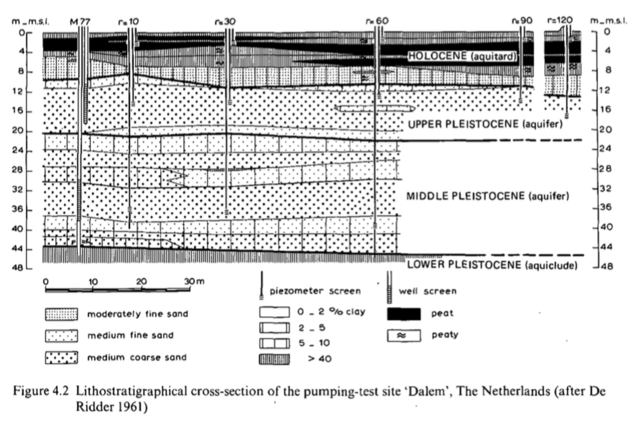
Fig. 53 Cross section pumping test Dalem (Kruseman & De Ridder, 1970, 1994)
The data are given below in a csv form:
t(min),s_piez1,s_piez2,s_piez3,t/(r1)^2,t/(r2)^2,t/(r3)^2,u,1/u,w(u)
,m,m,m,,,,,,
1,0.2,0.07,0,0.043252595,0.000307865,7.24049E-05,0.001,1000,6.33
2,0.25,0.08,0.03,0.08650519,0.000615729,0.00014481,0.001584893,630.9573445,5.87
3,0.24,0.1,0.03,0.129757785,0.000923594,0.000217215,0.002511886,398.1071706,5.41
4,0.27,0.1,0.05,0.173010381,0.001231459,0.00028962,0.003981072,251.1886432,4.95
5,0.27,0.11,0.05,0.216262976,0.001539324,0.000362024,0.006309573,158.4893192,4.49
6,0.26,0.1,0.06,0.259515571,0.001847188,0.000434429,0.01,100,4.04
7,0.27,0.11,0.05,0.302768166,0.002155053,0.000506834,0.015848932,63.09573445,3.58
8,0.28,0.12,0.06,0.346020761,0.002462918,0.000579239,0.025118864,39.81071706,3.13
9,0.29,0.13,0.06,0.389273356,0.002770782,0.000651644,0.039810717,25.11886432,2.69
10,0.28,0.14,0.07,0.432525952,0.003078647,0.000724049,0.063095734,15.84893192,2.25
11,0.3,0.13,0.08,0.475778547,0.003386512,0.000796454,0.1,10,1.82
12,0.27,0.14,0.07,0.519031142,0.003694377,0.000868859,0.158489319,6.309573445,1.42
13,0.3,0.13,0.08,0.562283737,0.004002241,0.000941264,0.251188643,3.981071706,1.04
14,0.28,0.11,0.09,0.605536332,0.004310106,0.001013669,0.398107171,2.511886432,0.71
15,0.3,0.12,0.08,0.648788927,0.004617971,0.001086073,0.630957344,1.584893192,0.43
20,0.3,0.14,0.09,0.865051903,0.006157294,0.001448098,1,1,0.22
25,0.3,0.13,0.09,1.081314879,0.007696618,0.001810122,1.584893192,0.630957344,0.09
30,0.32,0.15,0.1,1.297577855,0.009235941,0.002172147,2.511886432,0.398107171,0.02
35,0.31,0.17,0.11,1.51384083,0.010775265,0.002534171,3.981071706,0.251188643,0.00
40,0.32,0.13,0.1,1.730103806,0.012314588,0.002896196,6.309573445,0.158489319,0.00
45,0.33,0.16,0.13,1.946366782,0.013853912,0.00325822,10,0.1,0.00
50,0.32,0.18,0.14,2.162629758,0.015393236,0.003620245,15.84893192,0.063095734,0.00
55,0.35,0.18,0.11,2.378892734,0.016932559,0.003982269,25.11886432,0.039810717,0.00
60,0.34,0.17,0.13,2.595155709,0.018471883,0.004344294,39.81071706,0.025118864,0.00
75,0.34,0.17,0.14,3.243944637,0.023089853,0.005430367,63.09573445,0.015848932,0.00
90,0.35,0.18,0.14,3.892733564,0.027707824,0.006516441,100,0.01,0.00
105,0.35,0.18,0.14,4.541522491,0.032325795,0.007602514,,,
120,0.36,0.2,0.14,5.190311419,0.036943765,0.008688588,,,
135,0.35,0.19,0.13,5.839100346,0.041561736,0.009774661,,,
150,0.36,0.19,0.13,6.487889273,0.046179707,0.010860735,,,
165,0.35,0.19,0.15,7.136678201,0.050797677,0.011946808,,,
180,0.4,0.21,0.16,7.785467128,0.055415648,0.013032882,,,
195,0.36,0.2,0.16,8.434256055,0.060033619,0.014118955,,,
210,0.36,0.2,0.14,9.083044983,0.06465159,0.015205029,,,
225,0.36,0.21,0.15,9.73183391,0.06926956,0.016291102,,,
240,0.38,0.21,0.16,10.38062284,0.073887531,0.017377176,,,
270,0.39,0.22,0.15,11.67820069,0.083123472,0.019549323,,,
300,0.38,0.21,0.16,12.97577855,0.092359414,0.02172147,,,
330,0.36,0.22,0.16,14.2733564,0.101595355,0.023893617,,,
360,0.37,0.2,0.17,15.57093426,0.110831296,0.026065764,,,
390,0.39,0.21,0.16,16.86851211,0.120067238,0.028237911,,,
420,0.4,0.23,0.2,18.16608997,0.129303179,0.030410058,,,
450,0.38,0.23,0.17,19.46366782,0.13853912,0.032582205,,,
480,0.39,0.22,0.18,20.76124567,0.147775062,0.034754352,,,
510,0.38,0.22,0.17,22.05882353,0.157011003,0.036926499,,,
540,0.39,0.23,0.17,23.35640138,0.166246944,0.039098646,,,
570,0.39,0.2,0.18,24.65397924,0.175482886,0.041270793,,,
600,0.38,0.24,0.17,25.95155709,0.184718827,0.04344294,,,
1320,0.39,0.23,0.16,57.09342561,0.40638142,0.095574468,,,
1380,0.4,0.23,0.19,59.68858131,0.424853302,0.099918762,,,
1440,0.39,0.23,0.17,62.28373702,0.443325185,0.104263056,,,
1500,0.42,0.21,0.18,64.87889273,0.461797068,0.10860735,,,
1560,0.4,0.23,0.16,67.47404844,0.480268951,0.112951644,,,
1620,0.4,0.24,0.19,70.06920415,0.498740833,0.117295938,,,
1680,0.38,0.22,0.2,72.66435986,0.517212716,0.121640232,,,
1740,0.4,0.23,0.17,75.25951557,0.535684599,0.125984526,,,
1800,0.4,0.25,0.2,77.85467128,0.554156481,0.13032882,,,
1860,0.4,0.24,0.18,80.44982699,0.572628364,0.134673114,,,
1920,0.4,0.25,0.19,83.0449827,0.591100247,0.139017408,,,
2880,0.41,0.25,0.2,124.567474,0.88665037,0.208526111,,,
3360,0.39,0.23,0.19,145.3287197,1.034425432,0.243280463,,,
4320,0.4,0.23,0.18,186.8512111,1.329975556,0.312789167,,,
4800,0.4,0.23,0.2,207.6124567,1.477750617,0.347543519,,,
5760,0.38,0.23,0.18,249.1349481,1.773300741,0.417052223,,,
6240,0.38,0.24,0.17,269.8961938,1.921075802,0.451806575,,,
7200,0.39,0.23,0.18,311.4186851,2.216625926,0.521315278,,,
7680,0.38,0.23,0.2,332.1799308,2.364400988,0.55606963,,,
8640,0.39,0.22,0.17,373.7024221,2.659951111,0.625578334,,,
9120,0.39,0.23,0.18,394.4636678,2.807726173,0.660332686,,,
10080,0.4,0.23,0.19,435.9861592,3.103276296,0.72984139,,,
10560,0.41,0.24,0.17,456.7474048,3.251051358,0.764595742,,,
11520,0.4,0.24,0.19,498.2698962,3.546601481,0.834104446,,,
12000,0.41,0.24,0.19,519.0311419,3.694376543,0.868858797,,,
12960,0.41,0.25,0.19,560.5536332,3.989926667,0.938367501,,,
13440,0.39,0.23,0.17,581.3148789,4.137701728,0.973121853,,,
14400,0.39,0.22,0.19,622.8373702,4.433251852,1.042630557,,,
14880,0.4,0.23,0.16,643.5986159,4.581026914,1.077384909,,,
15840,0.39,0.24,0.19,685.1211073,4.876577037,1.146893613,,,
16320,0.39,0.23,0.17,705.8823529,5.024352099,1.181647964,,,
17280,0.41,0.25,0.19,747.4048443,5.319902222,1.251156668,,,
17760,0.4,0.22,0.19,768.16609,5.467677284,1.28591102,,,
18720,0.39,0.22,0.18,809.6885813,5.763227407,1.355419724,,,
19200,0.39,0.24,0.18,830.449827,5.911002469,1.390174076,,,
20160,0.38,0.24,0.19,871.9723183,6.206552593,1.45968278,,,
20640,0.39,0.24,0.18,892.733564,6.354327654,1.494437132,,,
21600,0.39,0.23,0.16,934.2560554,6.649877778,1.563945835,,,
22080,0.41,0.22,0.18,955.017301,6.797652839,1.598700187,,,
23040,0.4,0.22,0.17,996.5397924,7.093202963,1.668208891,,,
23520,0.4,0.23,0.18,1017.301038,7.240978025,1.702963243,,,
24480,0.41,0.25,0.2,1058.823529,7.536528148,1.772471947,,,
24960,0.4,0.23,0.19,1079.584775,7.68430321,1.807226299,,,
25920,0.4,0.24,0.18,1121.107266,7.979853333,1.876735002,,,
26400,0.38,0.23,0.18,1141.868512,8.127628395,1.911489354,,,
27360,0.4,0.23,0.18,1183.391003,8.423178518,1.980998058,,,
27840,0.38,0.24,0.19,1204.152249,8.57095358,2.01575241,,,
28800,0.39,0.25,0.18,1245.67474,8.866503704,2.085261114,,,
29280,0.4,0.23,0.19,1266.435986,9.014278765,2.120015466,,,
30240,0.4,0.24,0.18,1307.958478,9.309828889,2.189524169,,,
30720,0.41,0.23,0.17,1328.719723,9.457603951,2.224278521,,,
31680,0.4,0.23,0.19,1370.242215,9.753154074,2.293787225,,,
32160,0.41,0.24,0.19,1391.00346,9.900929136,2.328541577,,,
33120,0.4,0.24,0.19,1432.525952,10.19647926,2.398050281,,,
33600,0.39,0.23,0.18,1453.287197,10.34425432,2.432804633,,,
34560,0.4,0.22,0.17,1494.809689,10.63980444,2.502313337,,,
35040,0.4,0.23,0.2,1515.570934,10.78757951,2.537067688,,,
36000,0.41,0.22,0.19,1557.093426,11.08312963,2.606576392,,,
36480,0.39,0.24,0.18,1577.854671,11.23090469,2.641330744,,,
37440,0.4,0.23,0.18,1619.377163,11.52645481,2.710839448,,,
37920,0.41,0.24,0.21,1640.138408,11.67422988,2.7455938,,,
38880,0.4,0.22,0.2,1681.6609,11.96978,2.815102504,,,
39360,0.4,0.22,0.17,1702.422145,12.11755506,2.849856856,,,
40320,0.42,0.23,0.17,1743.944637,12.41310519,2.919365559,,,
40800,0.38,0.22,0.19,1764.705882,12.56088025,2.954119911,,,
41760,0.4,0.23,0.18,1806.228374,12.85643037,3.023628615,,,
42240,0.4,0.24,0.19,1826.989619,13.00420543,3.058382967,,,
43200,0.38,0.22,0.17,1868.512111,13.29975556,3.127891671,,,
43680,0.38,0.24,0.19,1889.273356,13.44753062,3.162646023,,,
44640,0.4,0.24,0.19,1930.795848,13.74308074,3.232154726,,,
45120,0.4,0.23,0.19,1951.557093,13.8908558,3.266909078,,,
46080,0.4,0.24,0.17,1993.079585,14.18640593,3.336417782,,,
46560,0.39,0.24,0.18,2013.84083,14.33418099,3.371172134,,,
47520,0.41,0.23,0.19,2055.363322,14.62973111,3.440680838,,,
48000,0.38,0.24,0.19,2076.124567,14.77750617,3.47543519,,,
48960,0.4,0.23,0.17,2117.647059,15.0730563,3.544943893,,,
49440,0.39,0.22,0.19,2138.408304,15.22083136,3.579698245,,,
50400,0.38,0.23,0.16,2179.930796,15.51638148,3.649206949,,,
50880,0.41,0.24,0.19,2200.692042,15.66415654,3.683961301,,,
51840,0.41,0.22,0.18,2242.214533,15.95970667,3.753470005,,,
52320,0.39,0.23,0.21,2262.975779,16.10748173,3.788224357,,,
53280,0.4,0.25,0.2,2304.49827,16.40303185,3.857733061,,,
53760,0.4,0.25,0.19,2325.259516,16.55080691,3.892487412,,,
54720,0.41,0.24,0.19,2366.782007,16.84635704,3.961996116,,,
55200,0.39,0.24,0.18,2387.543253,16.9941321,3.996750468,,,
56160,0.4,0.25,0.19,2429.065744,17.28968222,4.066259172,,,
56640,0.39,0.22,0.17,2449.82699,17.43745728,4.101013524,,,
57600,0.38,0.23,0.17,2491.349481,17.73300741,4.170522228,,,
58080,0.39,0.23,0.17,2512.110727,17.88078247,4.205276579,,,
59040,0.39,0.23,0.19,2553.633218,18.17633259,4.274785283,,,
59520,0.39,0.25,0.18,2574.394464,18.32410765,4.309539635,,,
60480,0.39,0.23,0.19,2615.916955,18.61965778,4.379048339,,,
60960,0.4,0.22,0.18,2636.678201,18.76743284,4.413802691,,,
61920,0.41,0.24,0.18,2678.200692,19.06298296,4.483311395,,,
62400,0.39,0.23,0.19,2698.961938,19.21075802,4.518065747,,,
63360,0.39,0.22,0.19,2740.484429,19.50630815,4.58757445,,,
63840,0.39,0.23,0.17,2761.245675,19.65408321,4.622328802,,,
64800,0.42,0.24,0.18,2802.768166,19.94963333,4.691837506,,,
65280,0.39,0.24,0.19,2823.529412,20.09740839,4.726591858,,,
66240,0.39,0.25,0.17,2865.051903,20.39295852,4.796100562,,,
66720,0.39,0.24,0.19,2885.813149,20.54073358,4.830854914,,,
67680,0.39,0.23,0.19,2927.33564,20.8362837,4.900363617,,,
68160,0.4,0.21,0.2,2948.096886,20.98405877,4.935117969,,,
69120,0.39,0.24,0.2,2989.619377,21.27960889,5.004626673,,,
69600,0.38,0.25,0.17,3010.380623,21.42738395,5.039381025,,,
70560,0.39,0.23,0.17,3051.903114,21.72293407,5.108889729,,,
71040,0.4,0.23,0.18,3072.66436,21.87070914,5.143644081,,,
72000,0.39,0.24,0.16,3114.186851,22.16625926,5.213152784,,,
72480,0.4,0.25,0.16,3134.948097,22.31403432,5.247907136,,,
73440,0.38,0.24,0.19,3176.470588,22.60958444,5.31741584,,,
73920,0.41,0.25,0.18,3197.231834,22.75735951,5.352170192,,,
74880,0.41,0.23,0.19,3238.754325,23.05290963,5.421678896,,,
75360,0.39,0.22,0.18,3259.515571,23.20068469,5.456433248,,,
76320,0.4,0.23,0.18,3301.038062,23.49623481,5.525941952,,,
76800,0.41,0.24,0.19,3321.799308,23.64400988,5.560696303,,,
77760,0.38,0.22,0.2,3363.321799,23.93956,5.630205007,,,
78240,0.4,0.24,0.19,3384.083045,24.08733506,5.664959359,,,
79200,0.38,0.23,0.18,3425.605536,24.38288518,5.734468063,,,
79680,0.4,0.23,0.18,3446.366782,24.53066025,5.769222415,,,
80640,0.39,0.24,0.18,3487.889273,24.82621037,5.838731119,,,
81120,0.39,0.24,0.18,3508.650519,24.97398543,5.873485471,,,
82080,0.41,0.22,0.18,3550.17301,25.26953556,5.942994174,,,
82560,0.39,0.23,0.18,3570.934256,25.41731062,5.977748526,,,
83520,0.41,0.23,0.18,3612.456747,25.71286074,6.04725723,,,
84000,0.38,0.23,0.17,3633.217993,25.8606358,6.082011582,,,
84960,0.41,0.25,0.19,3674.740484,26.15618593,6.151520286,,,
85440,0.42,0.23,0.19,3695.50173,26.30396099,6.186274638,,,
86400,0.41,0.24,0.18,3737.024221,26.59951111,6.255783341,,,
86880,0.41,0.24,0.18,3757.785467,26.74728617,6.290537693,,,