1. Nomenclature
1.1. General
- \(x,y,z\,\mathrm{\left[L\right]}\)
Coordinates. \(z\) is upward positive relative to top of model, sea level, ground surface, top of aquifer or any other suitable fixed datum elevation.
- \(r\,\mathrm{\left[L\right]}\)
Distance from the well or center of model in the case of axial symmetric flow. Also used for the radius of a capillary.
- \(R\,\mathrm{\left[L\right]}\)
Radius of influence, outer radius of circular aquifer or island.
- \(t,\,\Delta t\,\mathrm{\left[T\right]}\)
Time.
- \(A\,\mathrm{\left[L^{2}\right]}\)
Surface area.
- \(V\,\mathrm{\left[L^{3}\right]}\)
Volume.
1.2. Hydraulic and mechanical properties
- \(\mu\,\mathrm{\left[FT/L^{2}\right]}\)
Water viscosity, e.g. \(\mathrm{\left[Ns/m^{2}\right]}=\mathrm{\left[Pa\,s\right]}\)
- \(\kappa\,\mathrm{\left[L^{2}\right]},\,k\,\mathrm{\left[L/T\right]}\)
Permeability (independent of fluid) and hydraulic conductivity. \(k=\rho_{w}g\frac{\kappa}{\mu}\). Note that \(\kappa\) and \(k\) are vectors, i.e. they are direction dependent.
- \(c\,\mathrm{\left[T\right]}\)
Vertical hydraulic resistance of aquitards or a low-conductive layer, \(c=d/k_{v}\) with \(d\,\mathrm{\left[L\right]}\) the thickness of this layer and \(k_{v}\,\mathrm{\left[L/T\right]}\) its vertical hydraulic conductivity.
- \(S\,\mathrm{[-]}\)
Elastic storage coefficient \(\mathrm{\left[L^{3}/L^{2}/L\right]}\)
- \(S_{s}\mathrm{\left[L^{-1}\right]}\)
Specific elastic storage coefficient \(\mathrm{\left[L^{3}/L^{2}/L\right]}\)
- \(S_{y}\mathrm{\left[L^{-1}\right]}\)
Specific yield \(\mathrm{\left[L^{3}/L^{2}/L\right]}\). Specific yield is storage from draining pores.
- \(\alpha,\,\beta\,\mathrm{\left[L^{2}/F\right]}\)
compressibility of water and bulk porous matrix respectively. \(\beta=1/E\) where \(E\) is the compression modulus.
- \(E_{w},\,E_{m}\,\mathrm{\left[F/L^{2}\right]}\)
Compression modulus of water and porous medium respectively. \(E=1/\beta\), where \(\beta\) is the compressibility.
- \(\rho_{w},\,\rho_{s},\,\rho_{b},\,\rho\,\mathrm{\left[M/L^{3}\right]}\)
Density of water, solids, bulk porous medium respectively.
1.3. Heat properties and flow
- \(c,\,c_{w},\,c_{s}\,\mathrm{\left[E/M/K\right]}\)
Bulk heat capacity, heat capacity of water and solids. \(c=\epsilon c_{w}+\left(1-\epsilon\right)c_{s}\)
- \(\lambda,\,\lambda_{w},\,\lambda_{s}\,\mathrm{\left[E/T/L/K\right]}\)
Bulk, water and solids heat conductance, \(\lambda=\epsilon\lambda_{w}+\left(1-\epsilon\right)\lambda_{s}\)
- \(\epsilon\,\mathrm{\left[-\right]}\)
Porosity of the porous medium
- \(\mathbb{D}\,\mathrm{\left[L^{2}/T\right]}\)
For heat flow \(\mathbb{D}=\frac{\lambda}{\rho c}\), i.e. heat conductivity over bulk volumetric heat capacity of water plus medium, \(\lambda=\epsilon\lambda_{w}+\left(1-\epsilon\right)\lambda_{s}\) and \(\rho c=\epsilon\rho_{w}c_{w}+\left(1-\epsilon\right)\rho_{s}c_{s}\). For diffusivity in the context of groundwater flow see under Aquifer system.
- \(\mathbb{R}\,\mathrm{\left[-\right]}\)
Retardation, i.e. the factor by which transport of mass or heat is delayed relative to that of the pore water. It is the amount of mass or heat in the water over the total amount of mass or heat in the water plus sorbed to/in the grains. Hence for heat \(\mathbb{R}=\rho_{w}c_{w}\epsilon/\left(\rho_{w}c_{w}\epsilon+\rho_{s}c_{s}\left(1-\epsilon\right)\right)\) with indices \(w\) and \(s\) referring to water and grains respectively.
1.4. Aquifer system
- \(q,\,q_{x},q_{y},\,q_{z}\,\mathrm{\left[L/T\right]}\)
Specific discharge, which generally is direction-specific (a vector)
- \(Q\,\mathrm{\left[L^{3}/T\right],\,\left[L^{2}/T\right]}\)
Discharge. It can mean the total discharge over the thickness of the aquifer in a cross section \(\mathrm{L^{2}/T}\) or the extraction or injection of a well, in which case its dimension is \(\mathrm{L^{3}/T}\).
- \(N,\,\overline{N}\,\mathrm{\left[L/T\right]}\)
Net recharge and the time or space average net recharge respectively
- \(h\,\mathrm{\left[L\right]}\)
Phreatic head, in the case of a water table aquifer, the head relative to the bottom of this aquifer, i.e. the wetted aquifer thickness
- \(\phi\,\mathrm{\left[L\right]}\)
Head in semi-confined and confined aquifers, relative to some predefined datum, i.e. sea level.
- \(s\,\mathrm{\left[L\right]}\)
Drawdown, or head relative to initial situation (lower case \(s\))
- \(p,\,\sigma_{w},\sigma_{s},\sigma_{e}\,\mathrm{\left[F/L^{2}\right]}\)
Pressure, water pressure, total or soil pressure and effective pressure. \(\sigma_{t}\) also used for total pressure.
- \(H\,\mathrm{\left[L\right]}\)
Thickness of aquifer. Often used only for water table aquifer, sometimes for any aquifer.
- \(D\,\mathrm{\left[L\right]}\)
Total thickness of aquifer
- \(kD\,\mathrm{\left[L^{2}/T\right]}\)
Transmissivity of an aquifer. \(kH\) may be used in an water-table aquifer.
- \(T\,\mathrm{\left[T\right]}\)
Characteristic time of a dynamic groundwater system.
- \(\mathbb{D}\,\mathrm{\left[L^{2}/T\right]}\)
Diffusivity. For flow \(\mathbb{D}=\frac{kD}{S}\) for thermal flow \(\mathbb{D}=\frac{\lambda}{\rho c}\), see under Heat
- \(\lambda\,\mathrm{\left[L\right]}\)
Characteristic length or spreading length of a semi-confined aquifer system, i.e. \(\lambda=\sqrt{kDc}\) with \(kD\,\mathrm{\left[L^{2}/T\right]}\) the aquifer’s transmissivity and \(c\,\mathrm{\left[T\right]}\) the aquitard’s vertical resistance.
- \(R,\,R_{0}\,\mathrm{\left[L\right]}\)
Fixed radial distance to the center of axial symmetric flow system at which the head is fixed or zero.
- \(LE\)
[-] Loading efficiency, \(LE=\frac{\beta_{m}}{\epsilon\beta_{w}+\beta_{m}}\). Note that \(LE+BE=1\)
- \(BE\)
[-] Barometric efficiency. \(BE=\frac{\epsilon\beta_{w}}{\epsilon\beta_{w}+\beta_{m}}\). Note that \(LE+BE=1\)
1.5. Groundwater waves
- \(A\,\mathrm{\left[L\right]},\,B\,\mathrm{[L]}\)
Wave amplitude.
- \(L\,\mathrm{\left[L\right]}\)
Width of the groundwater system.
- \(a\)
Damping factor of groundwater head wave moving through the aquifer, caused by a kind of tide. \(a=\sqrt{\frac{\omega}{2\mathbb{D}}}\)
- \(\omega\,\mathrm{\left[T^{-1}\right]}\)
or rather radians per time. The angle velocity of the wave. Full wave time \(T=2\pi/\omega\)
- \(T\,\mathrm{\left[T\right]}\)
Cycle time, time of a full wave. \(T=2\pi/\omega\)
1.6. Physics, math and mechanics
- \(g\,\mathrm{\left[F/M\right]\mbox{, }\left[L/T^{2}\right]}\)
Gravity, acceleration in the Earth’s gravity field or the force with which the earth’s gravity field pulls at a unit mass at ground surface in the direction of the earth’s center.
- \(\gamma\,\mathrm{\left[F/L\right]}\)
Surface tension, cohesion in capillary systems.
- \(\mbox{IR}\left(\tau\right)\mbox{, }BR\left(\tau,\Delta\tau\right)\mbox{, }SR\left(\tau\right)\)
Respectively: Impulse response, Block response, Step response of a system. \(\Delta\tau\) step size, \(\tau\) lapsed time since event started. See chapter on convolution.
- \(\mbox{erfc}\left(u\right)\)
Complementary Error function, i.e \(\mbox{erfc}\left(u\right)=\frac{2}{\sqrt{\pi}}\intop_{u}^{\infty}e^{-\zeta^{2}}d\zeta\), and, therefore, \(\frac{d\mbox{erfc}\left(u\right)}{du}=-\frac{2}{\sqrt{\pi}}e^{-u^{2}}\)
- \(\mbox{W}\left(u\right)\)
Theis’ well function, for transient flow to a well in a confined aquifer, i.e. \(\mbox{W}\left(u\right)=\mbox{iexp}\left(u\right)=\intop_{u}^{\infty}\frac{e^{-\zeta}}{\zeta}d\zeta\), iexp is the exponential integral.
- \(\mathrm{W}\left(u,\frac{r}{\lambda}\right)\)
Hantush’s well function for semi-confined transient flow to a well, \(\mbox{W}\left(u,\frac{r}{\lambda}\right)=\intop_{u}^{\infty}\frac{1}{\zeta}\exp\left(-\zeta-\frac{1}{4\zeta}\left(\frac{r}{\lambda}\right)^{2}\right)d\zeta\)
- \(u\,\mathrm{[-]}\)
In 1D (cross sections as argument of the \(\mbox{erfc}\)-function), \(u=\sqrt{\frac{x^{2}S}{4kDt}}\). In axial symmetric situations, as argument of the Theis and Hantush solutions, \(u=\frac{r^{2}S}{4kDt}\)
- \(\mbox{I}_{o}\left(z\right)\mbox{, }\mathrm{I}\left(z\right)\mbox{, }\mathrm{K}_{o}\left(z\right)\mbox{, }\mathrm{K}_{1}\left(z\right)\)
dimensionless modified Bessel function using in axial-symmetric semi-confined steady-state solutions. They depend on the scaled distance \(z=r/\lambda\), with \(\lambda=\sqrt{kDc}\)
2. Introduction
This syllabus has been prepared as part of the IHE master’s program in Hydrology and Water Resources, at IHE Delft, The Netherlands. The part given by the author, i.e. transient analytical solutions, consists of a total of 18 lecture hours divided over four and a have days. The majority of ours will be oral lectures and a minority will be practical exercises in which the students learn to solve their problems by implementing the groundwater solutions in Python.
The material for this course will be stored on Github (https://github.com). Search for Theo Olsthoorn combined with github and or TransientGroundwater to find the site an or pictures of me. The material includes Jupyter notebooks that were used to generate most of the figures in this syllabus.
2.1. Objectives of the course
The students will become familiar with the basic 1D and axially symmetric transient groundwater solutions that can readily be applied in practical situations when a computer models is not readily available, where a fast idea of the effect of groundwater impacts is required, where a model is to be verified and so on.
Students will learn how to deal with and apply superposition, which is perhaps the most important tool to handle more complex systems with analytically.
Students will obtain insight in the transient behavior of groundwater systems, and learn to reason based on their characteristics such as halftime and the relations between parameters and the way parameters workout in the effect on the system.
Students will learn to simplify analytical solutions to extract behavior characteristics that are easy to understand and apply for under specified conditions.
Closed analytical solutions for transient groundwater flow are only available for linear systems, i.e. systems with a constant transmissivity and storativity. Students will learn how to deal in an approximate way with situations where transmissivity will vary due to extractions or injections of water.
Students will gain insight in the behavior of real-world groundwater systems and learn how to read their reaction.
Students will also learn what physics cause a given behavior of groundwater systems. Storage characteristics and barometric and tidal reactions will be dealt with.
Students will learn and exercise how to implement transient analytical solutions in Python and visualize their results.
Students will learn how to analyze basic pumping tests to obtain the parameter values of a groundwater system.
Depending on the group, students will learn how to handle complicated time varying systems by means of convolution.
Students will carry out an assignment in which they apply the various aspects they’ve learned.
2.2. Exam
The exam is closed-book and will last one hour. It consists of solving several tasks and providing answers to questions concerning the text. Required formulas will be given.
2.3. Assignment
An assignment will be provided. It can be partially made in class during the exercises in the afternoons. I must have the results when I judge your written exams, that is, by the end of the week in which the written exam takes place, simply because I can’t give marks without the assignments. Any assignments handed in thereafter will not be graded, which implies that the entire mark will be defined only by the results of the written exam.
It is clear that I expect everyone to do his/her own assignments. It is generally easy for me to see who copied his or her work from someone else.
2.4. Gradiing
Grading will be 70% for the exam, 30% for the assignments.
Answers given during the exam must show their motivation, that is, the rationale: I want to see what (mental) steps you make. So motivate each step with some clarifying words. Just numbers or incomprehensible formula derivations do not count!
2.5. What to learn / understand
Sections [chap:Introduction-to-transient] through [sec:Elastic-Storage]. Check yourself by answering the questions. Skip Earth tides (not for exam).
Sections [sec:Scope-5-1] through [sec:Sinusoidal-fluctuations], to the extent that you understand and can answer the questions in Questions.
Sections [subsec:Basins-of-half-infinite-lateral-extent] through [subsec:Questions-5-4-2]. Understand how the erfc function works, understand that that the differential equation is a water balance, and understand what the parameters in the solution mean. Answer the questions in Questions.
Skip Higher-order solutions (not for exam) and [subsec:Questions-5-4-4]; they may be useful as a future reference.
Superposition in time, half-infinite aquifer. Understand how superposition in time works, and how to apply it when the analytic solution is provided.
Sections [subsec:Introduction-5-5-1] through [subsec:Questions-5-5-5]. Understand how superposition in space works. Answer the questions of Questions.
Symmetrical drainage from a land strip bounded by straight head boundaries (characteristic time of flow basins). Understand what the formula in Analytical solutionmeans and how we cracked it down to a characteristic time for groundwater systems and to their halftime in Long-term drainage behavior, characteristic drainage time. Check if you can answer the questions in Questions.
Chapter [chap:Transient-flow-to-wells]: transient flow to wells.
Introduction and [sec:Wells-and-well]: introduction to wells.
General relation between the well-induced head change in a water-table and confined aquifer and the relation between the different analytical solutions for drawdown by a fully penetrating pumping well, Theis: Relation between the transient and steady-state well solutions. The Theis solution and its approximation.
It’s always good if you exercise to derive the basic differential equations (i.e. the physics) yourself. This is, in fact, a basic engineering skill as it specifies the physics of the problem. Realize that these partial differential equations are always water balances for an arbitrary, infinitesimally small portion of the aquifer.
Theis and Hantush wells in an infinite aquifer with constant transmissivity and storativity; the governing partial differential equation: Understand the situation covered by the Theis and Hantush solutions. Understand the behavior of these solutions on double log and half log axes. Understand where the extracted water comes from in both cases. Understand that Theis is a special case of Hantush. Understand how the simplified Theis solution is derived and why its useful. Understand the radius of influence. Understand the discharge at distance in the Theis case and what it implies. What are type curves?
Pumping-test analyses Pumping tests: Understand the concept of a pumping test. The interpretation of a pumping test in the Theis situation using the simplified logarithmic approximation of the well function (the trick to always determined the transmissivity from the drawdown per log-cycle of time. The way to determine the storage coefficient using the simplified log-approximation of the Theis function and it is limitation (partial penetration, clogged pumping well when measuring when measuring level inside the pumping well).
Understand the principle of the classic analysis of pumping tests in the Theis and Hantush situation using graphs and type curves on double logarithmic scales (or paper).
Partial penetration of well screens Partial penetration of the well screen in the aquifer: Just understand what it is and what effect it has on the drawdown near the well. You an always use this section as a reference in the future. Only understand the mechanism, as you are likely to encounter it in practice.
Chapter [chap:Convolution] Convolution: Understand what convolution is. Convolution is extremely useful as it allows to simulate groundwater with simple formulas for arbitrarily varying input in an efficient and very general way. It can be seen as a smart form of superposition.
Chapter [chap:Laplace-solutions] Laplace solutions: Skip. May be used as a reference.
2.6. Note with respect to the exercises
Nowadays, there are two skills that students should acquire to be able to do sound quantiative analysis like it is the case in this course: Python and QGIS. My motivation is as follows:
With Python, there is no limit to what you as student of professional may compute (and visualize) on your laptop,. Neither is there any practical limit to the amount of data you can handle and process, or the complexity you can handle. And, perhaps the best of it: it is free of charge.
With QGIS there is no limit to the spatial data you can handle, analyze and process. And it is also free of charge.
With these two tools you equip yourself for the future as an engineer or scientist. Both Python and QGIS are free, which is a unique feature of our time. Never before was so much computing power available to everybody. And, nobody can ever take it from you, just because it’s free, always present for you to exploit it on your own laptop. Therefore, it is only up to you yourself to acquire the skills to use it. To help you, there is an immense amount of resources and information on the internet about both these tools, so you should never be without an answer to your questions. There are also numerous tutorials on the Internet, both written and on video, and, of course, there exists a large pile of books. Python and QGIS, which have been widely around for only about 1.5 decades, have already changed the world for engineers and scientists and are continuing to do so every day. So if you don’t want to be left behind, pick it up. My advice to you, dear students, is to start using both Python and QGIS for all your projects from now on.
The exercises for this course will be done in IPython notebooks (now called Jupyter notebooks), which are a terrific means to communicate your work with others, including your teachers. These notebooks, which were originally developed for Python only, have since a few years been extended to over 47 other computer languages, like R and Julia. That is why the name was changed from IPython notebooks to Jupyter notebooks. These notebooks allow you to combine, text, formulas and code, neatly formatted, while computations are done and visualized within the notebook itself. Therefore, if your notebook is correct, then your work is correct. And because the text, with formulas, code and graphical results can be nicely formatted within the notebook, the notebook is also a great means for sharing your results as a living document or, if you like, as a pdf document, which you can send to your teacher if he/she does not have or know Python.
To convince yourselves read what Nature (world’s most famous scientific journal) said about Ipython notebooks in 2014:
https://www.nature.com/news/interactive-notebooks-sharing-the-code-1.16261
If you want some examples and tutorials see:
https://github.com/Carreau/iPython-wiki/blob/master/A-gallery-of-interesting-IPython-Notebooks.md
https://github.com/iPython/iPython/wiki/A-gallery-of-interesting-IPython-Notebooks
Just do a few of the examples. You’ll see that you can reach out over the entire internet, and could even embed a live webcam from home (or from your data loggers, of course) in your own notebook.
For exploratory computing, which is what you’ll be doing most of the time, see: Search for Exploratory computing Mark Bakker to find his github site from which you can copy the tutorial examples that he uses to teach Python to 2nd year students of the TUDelft.
A Jupyter notebook implies: 1) Rich web client. 2) Text and Math 3) Code 4) Results 5) Share and reproduce
For this see
See https://www.dataone.org/sites/default/files/sites/all/documents/perez2017webinar_sm.pdf
—
Theo Olsthoorn, Dec. 2017/ Jan 2021/ May 2022
3. Introduction to transient phenomena in groundwater
Transient phenomena can only occur if there is some form of storage for water under pressure. Without storage, at least theoretically, all changes of water pressures would spread out with infinite speed across the entire medium. The studied system would then always be in steady state. Clearly, this is never the case in physical reality. Every groundwater system has ways to store and release water under changes of pressure. The specific change of water volume in the porous medium per unit change of pressure (or head) determines the transient behavior of the groundwater system.
Under confined groundwater-flow conditions, part of the storage comes from compressibility of the porous medium and part from the compressibility of the water. Under conditions of a free water table, i.e. under unconfined flow conditions, meaning when a free water table is present, also called phreatic groundwater, most storage comes from filling and emptying pores above the water table and only a minor part from elastic storage. The elastic storage is about two orders of magnitude smaller than the phreatic storage. Because of this, elastic storage is mostly neglected for aquifer systems with a free water table.
Groundwater systems can be very slow and very fast. Whether a groundwater system is slow of fast depends on factors that we will study later in Long-term drainage behavior, characteristic drainage time. An example of a very slow groundwater system, one that takes tens of thousands of years to reach equilibrium, is presented in Fig. 3.1, which shows the ongoing decay of the groundwater mound in the Kalahari Desert since the last wet episode, which happened some 12500 years ago (Vries 1984). The line along which the cross section was made is shown in Fig. 3.2 together with the elevation profile.
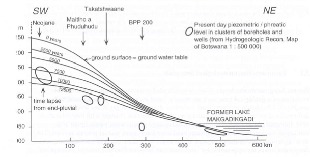
Fig. 3.1 Gradual decay of the water table in the Kalahari Desert (Vries 1984).
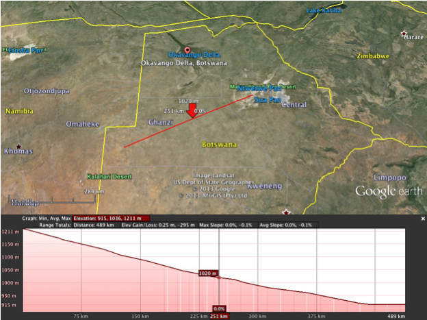
Fig. 3.2 Approximately 500 km long cross section studied by (Vries 1984), the water table of which is shown in Fig. 3.1
Dynamics of groundwater may also be divided into reversible and irreversible behavior. In this syllabus, we will deal with reversible systems only. Forms of irreversible storage may nevertheless be important under specific circumstances, or may even be quite common. Therefore, we will start with an illustration of some forms of irreversible transient behavior of water-filled porous media.
4. Irreversible transient phenomena
4.1. Consolidation
One possible form of volume change is due to reordering of ground particles, which may happen due to an increase of the effective pressure (= grain pressure), and is characterized by the squeezing out water which leads to an irreversible decline of pore space. This phenomenon is called consolidation and leads to land subsidence. The effective stress, \(\sigma_{e}\), is the pressure transmitted between the grains. Consolidation is especially well known for clay. In clay, under increased effective stress, micrometer-scale clay plates get reordered and the pore space thus becomes irreversibly smaller.
As long as grain stresses on vertical planes are horizontal, as is the case in undisturbed horizontal sediments, the total vertical stress, \(\sigma_{z}\), (in following chapters we will often use the symbol \(p\) instead of \(\sigma_{e}\), but they are the same), working on a horizontal plane in the subsoil always equals the total weight above this plane. This weight includes possible loads on ground surface. The total vertical stress \(\sigma_{z}\) itself is the sum of the water pressure, \(\sigma_{w}\), and the effective vertical stress \(\sigma_{e}\)
If we increase the vertical stress, for instance by loading the surface with a layer of sand, or by filling a surface reservoir, or due to rainwater infiltrating during the winter season, both stresses will change
If the water pressure changes, while the total weight remains constant, as is the case when we lower the head in a confined aquifer (reflect on why this must be so?), then the water pressure and the effective stress are directly related
Therefore, if we lower the head, i.e. the water pressure, the effective stress increases and the water pressure decreases. This works the other way around in case the head were increased instead of lowered.
It follows that the lowering of the water pressure puts the grains of the porous medium under higher stress, which may, therefore, lead to (irreversible) subsidence in vulnerable soils.
An increased effective stress causes a reduction of the volume of the porous medium and, therefore, also of its pore space. To compensate for this reduced space, water will be squeezed out. The speed at which this happens depends on the conductivity of the compressed layer as well as its thickness, as with thicker layers it takes more time for the compressed water to reach the top or bottom of the layer, from which the water could escape.
Large-scale groundwater extractions have, therefore, led to large subsidences affecting large areas in, among others, Mexico, USA and the UK (Fig. 4.1).
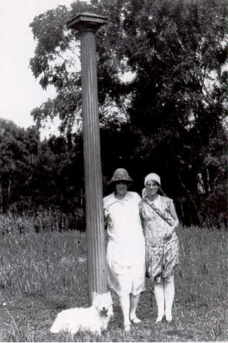
Fig. 4.1 Over \(3\mbox{m}\) subsidence in the UK

Fig. 4.2 Rising sea level since the year 1000 with tide fluctuation curve and subsidence (descending curve) all relative to mean sea level (about NAP in the figure). Also shown are water management technologies available over time (Dufour 2000)
Subsidence can be relatively fast (happening within weeks) or slow (taking place over centuries) on local to regional scales.
Subsidence also occurs as a result of drainage of wetlands and peat areas. Peat means organic soil, which can decay. This lowering of the shallow water table also increases the effective stress as we saw above. This subsidence is especially evident in a low country like the Netherlands, where drainage of wetlands by ditches has taken place for about thousand years.
With regard to organic soils, called peat, it is not only the increase of the effective stress caused by drainage that causes the subsidence. It is also the entry of oxygen that can enter peaty soils when they are drained. This oxygen causes oxidation (a kind of natural burning) of the peat, giving an extra boost to the subsidence. Subsidence caused by oxidation may continue until it all peat has disappeared!
The peaty areas in the west and north of the Netherlands have thus subsided several meters (Fig. 4.2). This is why about half the Netherlands lies nowadays below sea level.
In case the original soil layers consisted of alternations of peat and clay, as they often do, the shallow subsoil will consist more and more of pure clay at the top where all peat was burnt away by oxidation, with the original mixture still present below the water table. This clay layer at the top is the collection of all the clay that was present in the original profile, which may have been several meters thick.
4.2. Liquefaction
Another irreversible phenomenon involving reordering of grains, is known as liquefaction, which can happen very fast and spectacularly. Liquefaction is associated with pressure waves, or shocks. Fine sand may have been at rest for thousands of years, even with its pore space being greater than according to the most dense packing of the grains. In the case of a shock, for instance due to an earthquake, the sudden change of water pressure may be so great as to cause the effective stress to be zero for a fraction of a second, during which the grains lose their mutual friction. The ground then loses its internal friction and momentarily turns into a quicksand. In fact, it suddenly becomes a dense liquid in which grains float as freely moving particles. The matrix will resettle within minutes at a smaller overall volume. During this resettling, the pore water no longer fits between the grains in their denser packing. As soon as the surplus water has escaped the soil resettles and everything sunk into the heavy liquid is stuck forever (see Fig. 4.3).
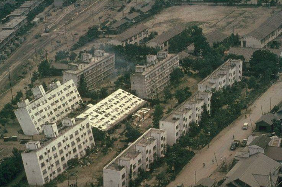
Fig. 4.3 Liquefaction in the USA (see http://www.ce.washington.edu/~liquefaction)
4.3. Intrusion of salt water
In many regions, especially deltaic regions, fresh groundwater floats on saline water, which is heavier (denser) than fresh water. (The difference in density between fresh and ocean water is about 2.5%). The fresh groundwater in the Netherlands is largely floating on salt water as is shown in the cross section in Fig. 4.4. It will generally take several hundred years to a thousand years for a freshwater lens to build up from natural precipitation. The equilibrium may easily be disturbed by extraction of fresh water, but also by construction of harbors, canals and polders. This will cause upconing of salt water from below and lateral intrusion of salt water into aquifers along the coast. Given the time it takes to restore such systems under natural conditions, mining of these systems may be considered irreversible under many practical situations as there are no real means (or sufficient fresh water) to restore the systems within the time horizon of a generation. Good groundwater management is, therefore, essential, but hard to realize in situations of water scarcity.
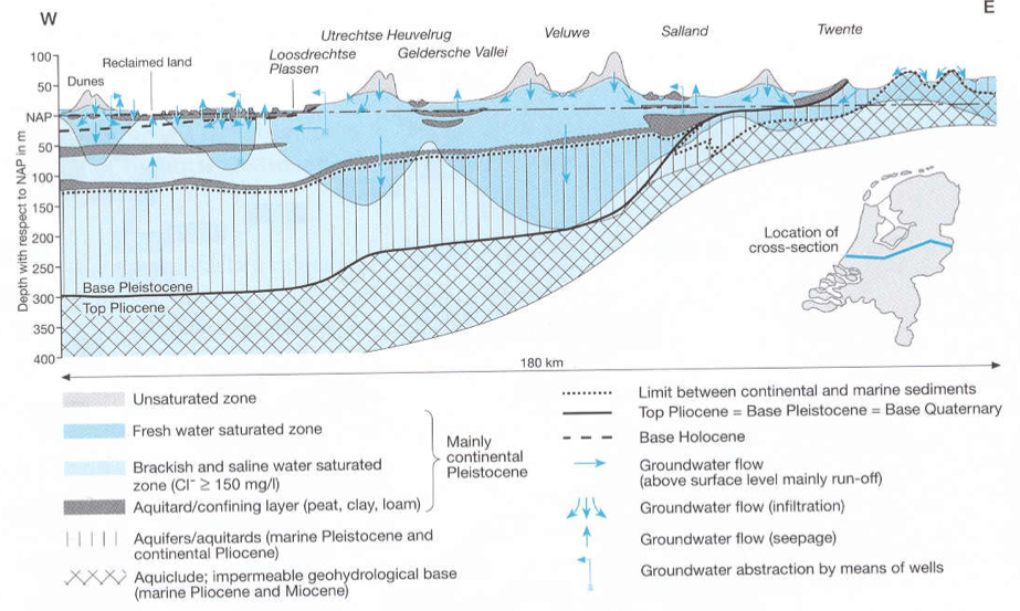
Fig. 4.4 Dynamically floating fresh water on salt water in the cross section through the Netherlands. The interface may take hundreds of years to reach its equilibrium. It will continuously adapt to changing circumstances such as climate and sea level rise, as well as to artificial changes in the water cycle (Dufour 2000).
4.4. Questions
Mention some processes due to which the subsurface may lose water irreversibly.
Explain how these processes work, i.e. what the mechanisms behind them are, and under which preconditions they occur.
Why would one argue that extraction of fresh water from a freshwater body that floats on salt water is irreversible?
5. Reversible groundwater storage
In the remainder of this syllabus, we will restrict ourselves to reversible groundwater storage phenomena, i.e. phenomena in which the porous medium is not changed.
In groundwater flow systems, three separate forms of storage may be distinguished:
Phreatic storage, which occurs in unconfined aquifers, i.e. aquifers with a free water table. It is due to filling and emptying of pores at the top of the saturated zone.
Elastic storage, which is due to combined compressibility of the water, the grains and the porous matrix (soil skeleton). This storage releases or stores water wherever the pressure changes.
Sometimes, the interface between fresh water and another fluid (be it saline water, oil or gas) can provide a third type of storage. This works by displacement of the interface, generally between the fresh water and the saline water. When displacing an interface, the total volume of water in the subsurface remains essentially the same, however, the amount of usable fresh water may increase (or decrease) at the cost of saline water, and therefore, one may consider this storage of fresh water.
5.1. Phreatic storage (water table storage, specific yield, Sy)
Phreatic storage is due to the filling and emptying of pores above the saturated zone, i.e. above the water table. Because it is related to changes of the water table, it is limited to phreatic (unconfined) aquifers.
The storage coefficient for an unconfined aquifer is called specific yield and is denoted by the symbol \(S_{y}\). It is dimensionless, as follows from its definition
where \(\partial V_{w}\) is the change of volume of water from a column of aquifer per unit of surface area and \(\partial h\) is the change of the water table elevation.
\(S_{y}\), therefore, is the amount of water released from storage per square meter of aquifer per m drawdown of the water table.
Hydrogeologists, and groundwater engineers alike, often treat specific yield as a constant. In reality, the draining and filling of pores is more complex and this should be kept in mind in order to judge differences of \(S_{y}\) values under different circumstances even with the same aquifer material. This will be explained further down.
There is no such thing as a sharp boundary between the saturated and the unsaturated porous medium above and below the water table. In fact, the water content is continuous across the water table.
The water table is, by definition, the elevation where the pressure equals atmospheric pressure.
Because we relate all pressures relative to atmospheric, we may say the water table is the elevation where the water pressure is zero (relative to the pressure of the atmosphere).
The simplest conceptual model for the zone above the water table is a vertical straw or radius \(r\) standing with its open end in water. Due to adhesion between the water and the straw, the water level will be sucked upward in the straw against gravity, thereby reaching an equilibrium height \(h\) as shown in Fig. 5.1.
The soil itself may be considered to consist of a dense network of connected tortuous pores of small but widely varying diameter that may be fully or partially filled with water. Due to adhesive forces, pores may even be fully filled above the water table.
In pores above the water table the pressure is negative (i.e. below atmospheric).
If grains can be wetted (attract water), as is generally the case with water, water will be sucked against gravity, into the pores above the water table over a certain height. This height mainly depends on the diameter of the pores.
One can immediately compute the equilibrium of the water in the pore. We have gravity pulling down the water column reaching above the water table, and we have the cohesion force. Hence,
where \(\rho\) [kg/m \(^{3}\)] is the density of water, \(g\) [N/kg] is gravity, \(\gamma\) [N/m \(^{2}\)] is the cohesion stress, and \(\alpha\) the angle between the cohesion stress and the vertical. Hence,
which shows that the suction height \(h\) is proportional to \(1/r\), the inverse radius of the straw.
In practical situations, \(\alpha\) is small so that \(\gamma\cos\alpha\approx\gamma\). As \(\gamma\) points is in the direction of the surface tension \(\tau\) (see Fig. 5.1) where the water surface meets the wall of the straw, we also have
with \(\tau\) the surface tension of the water surface, which equals \(\tau=75\times10^{-3}\mathrm{N/m}\), see any physical handbook or look it up on Wikipedia. Therefore, we can compute the suction head \(h\) immediately given a pore radius.
Numerically,
If we express \(h\) and \(r\) in mm, (using \(h^{*}\) and \(r^{*}\) to indicate mm), we get
This implies that water in a pore of 1 mm radius may be sucked up over about 15 mm, and water in a pore with a radius of 0.1 mm over 15 cm and water in a pore with a radius of 0.01 mm radius over 1.5 m. In reality, the suction may be 50% smaller because of the angle \(\alpha\) that was ignored here.
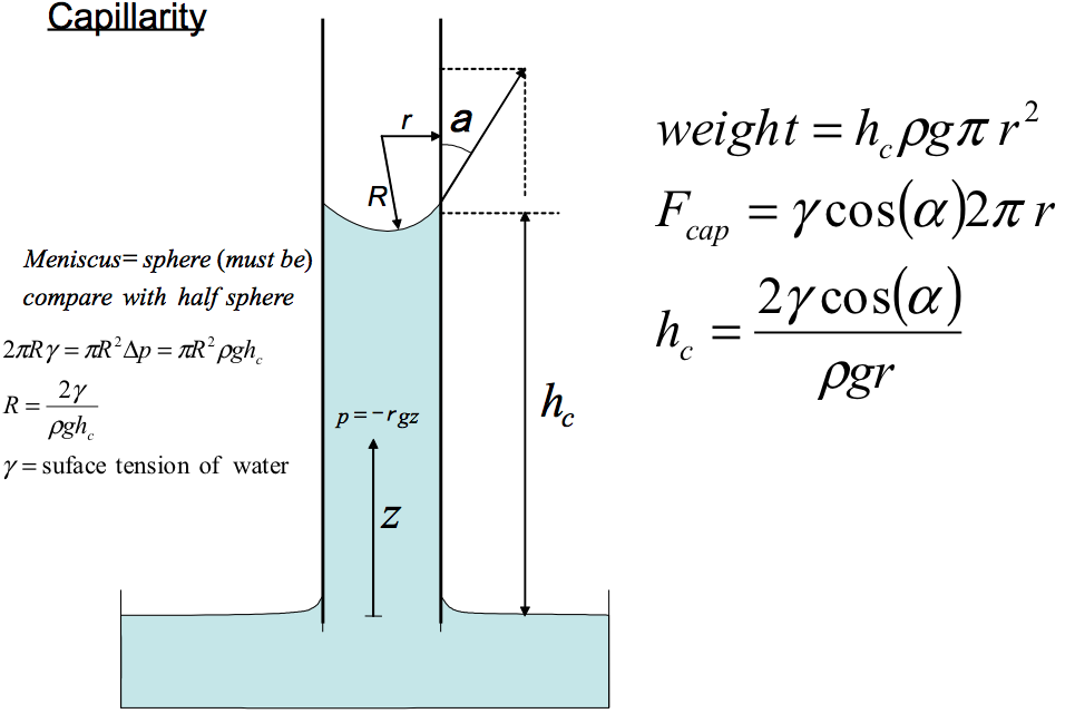
Fig. 5.1 Straw of radius \(r\) representing a pore connected to the water table

Fig. 5.2 A porous medium imagined as a large set of pores of varying diameter
A porous medium has pores of varying diameter, which may conceptually be imagined as in Fig. 5.2. This implies that the line of filled pores will not be sharp. Therefore, the saturation above the water table will gradually decline as shown in the right-hand figure .
The diameter of the widest pores will determine the height fully saturated above the water table, i.e. the thickness of the so-called capillary fringe. In gravel, the capillary fringe will be almost zero, but it may be several decimeters or even meters thick in fine-grained materials such as fine sand, loess, loam and clay. In sands, the capillary zone is usually 15-30 cm thick, depending on the grain size. The thickness of the capillary zone is sometimes visible as a wet zone in the banks of surface water. Note that all water above the water table is under negative pressure.
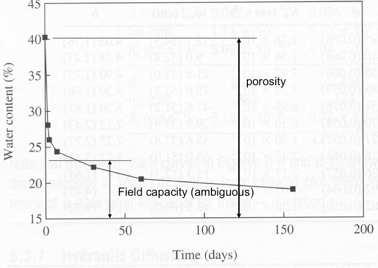
Fig. 5.3 Drainage of water from column after lowering the water table
When the water table is lowered, for instance in a column of sand, and we measure the amount of water drained over time, we see that drainage is not immediate (Fig. 5.3). After a couple of days, the drainage rate becomes negligibly small. We may thus call the amount drained during a couple of days the specific yield. It is immediately obvious that specific yield is not a unique physical parameter. The more time we take, the higher the specific yield becomes. It implies that the duration of the test determines the value to some extent. It also implies that a specific yield, when determined from a pumping test of a couple of days duration, is likely to be smaller than that determined from the seasonal fluctuation of the water table.
While the amount of water drained from the subsurface due to lowering of the water table is called specific yield, the amount retained is the soil is called the specific retention. Together they add up to the soil’s porosity (Fig. 5.4). Specific retention is essentially the same as the so-called field capacity, i.e. the amount of water the soil can hold against gravity. It is defined is the amount of water retained in an originally saturated soil sample after a few days of free drainage at a suction head of about 200 cm.

Fig. 5.4 Relation between grain size, porosity, specific yield and specific retention (Bear 1988).
The porosity of porous materials varies, but that of sands is often about 35%. Fine sands tend to have somewhat higher values, while coarse sands tend to have somewhat lower porosities (see Fig. 5.4). This is related to the ease of compaction at the original time of sedimentation. Smaller grains have a higher surface area and are, therefore, more difficult to compact. In natural gravels, the pore space is often filled by finer grains. This reduces the porosity further. Fig. 5.4 shows that for very fine sands, the specific yield declines despite the higher porosity. This is mainly due to the higher specific retention (field capacity) of the finer-grained materials (Fig. 5.5) as well as to the lower hydraulic conductivity of such fine materials, and, therefore, further reduces their specific yield.
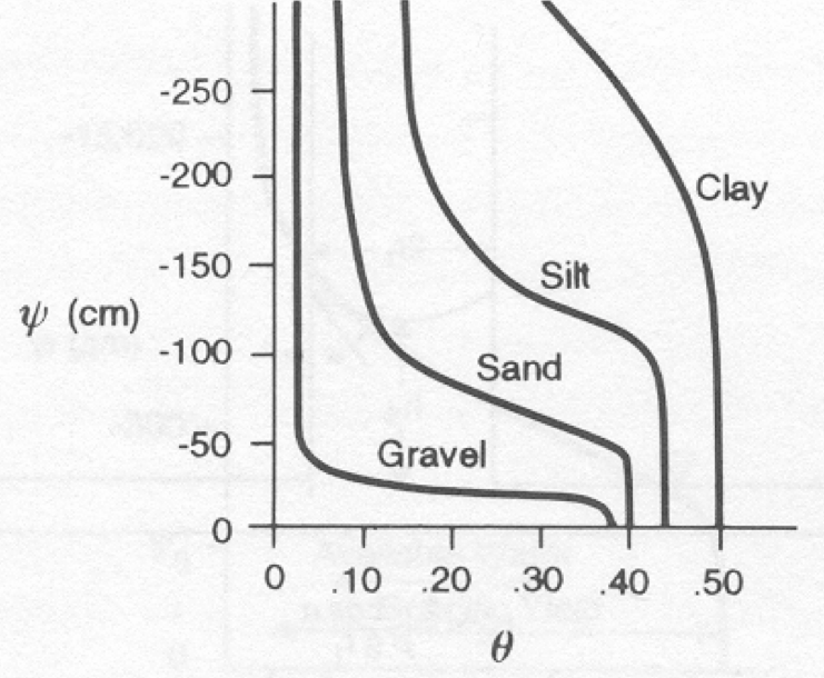
Fig. 5.5 Moisture content versus pressure head \(\Psi\), moisture retention curves (Bear 1988).
The behavior of water in the unsaturated zone is determined largely by the soil’s moisture retention curve of which a number is sketched in Fig. 5.5 (For the moisture retention curves of the Dutch soils see (Wösten, Veerman, and Stolte 1994).
These curves relate the moisture content to suction head, i.e. the negative head in the pores. Fig. 5.5 gives the general shape of these curves for typical soil materials. Therefore, in the case of perfect equilibrium between suction and gravity, the moisture characteristic curves represent the moisture content in the soil above the water table. The moisture content at 200 cm suction is generally taken as the field capacity. For sandy soils, the moisture content at this suction head is a good measure of the amount of water the soil can hold against gravity under free drainage conditions.
This implies that the moisture content depends on the distance to the water table (i.e. the suction). Hence, the ground surface above a shallow water table tends to be wetter than above a deep water table under otherwise the same circumstances. This must influence the specific yield as illustrated in Fig. 5.6.
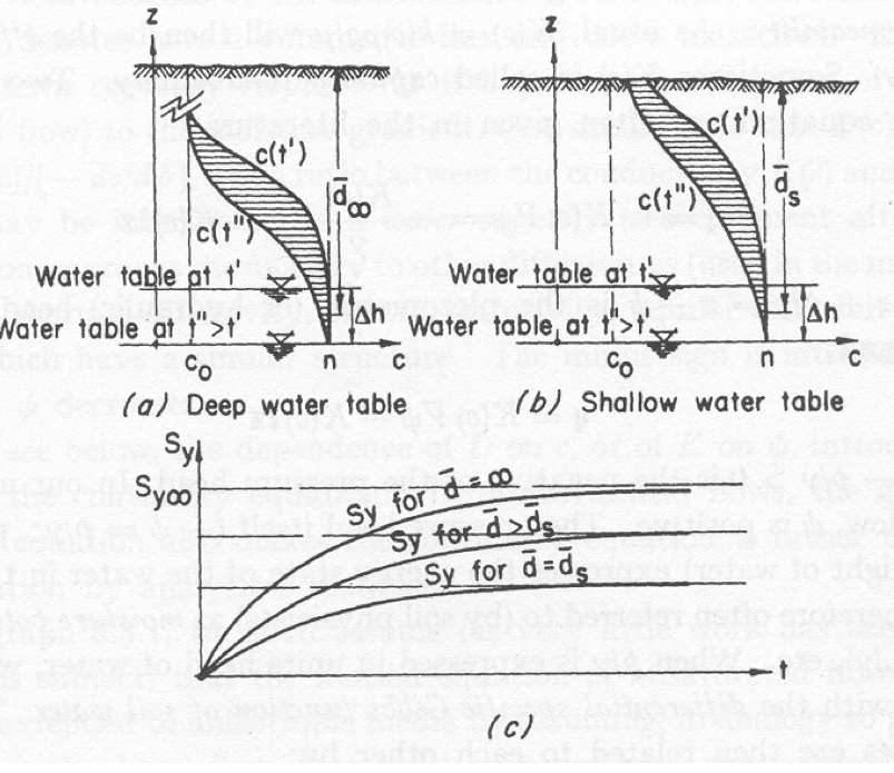
Fig. 5.6 Influence of depth and time on specific yield (Bear 1988).
When the water table is lowered, the entire moisture retention curve is lowered as is shown in Fig. 5.6-a. The specific yield times the difference of the two water tables equals the water from the hatched area times. It demonstrates that the entire unsaturated profile is involved in the specific yield. As already mentioned and shown in Fig. 5.6-c, specific yield increases with available drainage time.
If the water table is shallow (and the soil material is fine), a major part of the moisture retention curve will be cut off at ground surface as is shown in Fig. 5.6-b. Lowering of the water table will thus miss a portion of the hatched area of Fig. 5.6-a. Therefore, the specific yield is smaller the shallower the water table is. This is also shown in Fig. 5.6-c.
We should thus not be surprised to find that the same fine dune sand may have a specific yield of 22% inside a large dune area, where the water table is usually several meters below ground surface, and only 8% in an adjacent flower bulb field with the same sand, but with a water table of only 60 cm below ground surface.
Soil characteristics may vary between wide limits. Generally, the coarser the soil, the thinner the capillary fringe (see Fig. 5.5). A complication is that the moisture characteristic curves differ during wetting and drying. This phenomenon is called hysteresis, but this is beyond this course.
Groundwater hydrologists dealing with saturated groundwater usually just use a single constant value for the specific yield in their formulas and models. The specific yield can be estimated from the soil in question, from moisture characteristic curves, in the laboratory, from field measurements, from pumping tests or groundwater-model calibration.
Even though this approach may seem doubtful or just wrong in the eyes of some, using a constant but appropriately chosen specific yield works remarkably well in practice. It is more a matter of realizing oneself when a constant specific yield of a certain value is not applicable. The above outline is meant as a help in deciding on this and to consciousness about what is behind this“simple” hydrologic parameter that we denote by the symbol \(S_{y}\).
Some groundwater models, like MODFLOW, have an option to vary specific yield automatically with water-table depth.
5.1.1. Phreatic responses
By sensitive continuous measurements of the phreatic head, daily variations in evapotranspiration can be often determined. While in the past the groundwater head could be gauged continuously on paper only, modern head loggers may register the head at short regular intervals and store large amounts of data internally for later use. With such instruments, accurate data become widely available and allow more detailed views on phenomena to be studied and analyzed. Such measurements are already known from Todd (1959) also printed in Todd and Mays (2005). Fig. 5.7 shows the daily fluctuation of the water table due to daily evapotranspiration measured more than sixty years ago. However, we find such fluctuations in all frequent registrations of shallow water tables under summer circumstances.
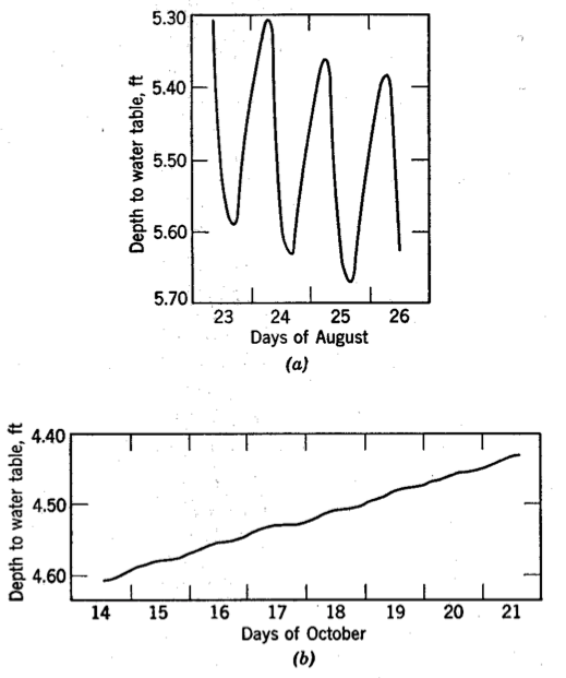
Fig. 5.7 Measured water-table fluctuations due to evapotranspiration variations (Todd and Mays 2005).
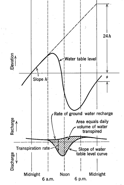
Fig. 5.8 Determining the evapotranspiration from water-table variations and a given specific yield (Todd and Mays 2005).
If the specific yield is known, evapotranspiration rates can sometimes be determined from such water-table registration. This can be demonstrated on the hand of these old measurements (Fig. 5.7 and Fig. 5.8). The groundwater balance at this point may be expressed as
where \(\overline{N}\) is the long-term trend of the net water-table recharge (positive or negative, i.e. precipitation minus evapotranspiration from the water table). \(N\left(t\right)\) is the short-term variation (during the day). So if one plots the derivative of the water table in a point versus time, it may be split into a more or less constant (long-term) trend and a the remainder due to short-term (daily) variation. If this short-term variation can be attributed to evapotranspiration from the water table, as it obviously is the case in the figure , one may determine it by taking the surface area between the measured head curve and its long-term trend, multiplied by the specific yield (hatched surface in Fig. 5.8[fig:water-table-fluctuation-due-to-evapotranspiration-1]).
5.1.2. Questions
What is the dimension of specific yield? What is the dimension of the elastic storage coefficient. What is the dimension of the specific storage coefficient?
How do specific retention, specific yield and porosity relate to each other?
How does porosity relate to grain size in general, and what is the reason?
Given another term for specific retention, one that is generally using in agriculture.
How does specific retention relate to grain size?
If the water table is lowered, which water is released around or above the water table?
What is the definition of the unsaturated zone?
Is it likely that the water from a rain shower easily infiltrates through worm and rabbit holes? If so explain why. If not also explain why?
What is a probable value for specific yield in a sand with porosity of 35%? And why?
How does capillary zone relate to air-entry pressure?
What is actually measured with the air-entry pressure?
How does the specific yield relate to the depth of the water table?
Using the model of a straw, how does capillary rise relate to the straw radius and the water surface tension?
Given a grain diameter of 0.2 mm, a radius that is 1/7th of this radius, and a water surface tension \(\gamma=75\times10^{-3}\mathrm{N/m}\), what would be the capillarity rise if the angle of the water surface and the straw is assumed to be zero?
5.2. Elastic Storage
5.2.1. Introduction
Till now, we only considered storage at the water table and gave very simple, but practical examples largely ignoring spatial dimensions. Spatial dimensions will be dealt with later. In this section, we handle the physics of elastic storage and will give some interesting everyday examples that are sometimes easily overlooked.
Elastic storage is the only storage occurring in confined and semi-confined aquifers, i.e. in aquifers without a water table, meaning aquifers that are completely filled with water from floor to ceiling. In such aquifers, we have no lowering of the water table whatsoever, unless the head is lowered to beneath the ceiling of the aquifer, a case further ignored here.
Therefore, in confined aquifer storage can only result from compression of the water and depression of the aquifer. The compressibility of the water and the grains themselves is quite obvious, but often the less obvious storage is the most important part. This is the deformation of the soil skeleton, the bulk matrix or the (bulk) porous medium as it is called.
5.2.2. Loading efficiency
To analyze the physics of elastic storage, we start with noting that the total load at any depth is carried by the total (vertical pressure) \(\sigma_{z}\) or \(p\,\mathrm{N/m^{2}}\). This total pressure must equal the sum of the vertical grain pressure (the so-called effective stress, \(\sigma_{e}\)) and the water pressure \(\sigma_{w}\)
This is indicated in Fig. 5.9. The brown horizontal beams and the springs in this figure are imaginary; they replace the volume \(V_{0}\) ( \(1\mathrm{m^{3}}\) say) that has been cut out of the aquifer. The two imaginary springs have the same properties as the water and the porous medium respectively. Let us see what happens when the pressure is increased by \(\Delta p\).
In that case, the volume (or height) \(V_{0}\) is reduced by \(\Delta V\) and the springs pressures are increased by \(\Delta\sigma_{w}\)and \(\Delta\sigma_{e}\) respectively. The springs have a different stiffness, so \(\Delta\sigma_{w}\ne\Delta\sigma_{e}\). However, each string will always carry a fixed proportion of the total stress. Therefore, we may write
where \(LE\) is this fixed proportion and is called the loading efficiency. The \(LE\) must obviously lie between \(0\) and 1 and is fixed for any particular porous medium. So if we put a weight, like a layer of sand, on ground surface, \(p\) in Fig. 5.9 will increase by \(\Delta p\), a change that is equal to the weight of the layer of sand per \(\mathrm{m}^{2}\) placed on ground surface. We may then say \(\Delta\sigma_{w}=LE\,\Delta p\), where the loading efficiency \(LE\) is a fixed number between 0 and 1, specific to a aquifer in question. If we have a piezometer in the aquifer, we’ll notice that the water level (hence, the head) has risen by placing the sand on ground surface. The head rise is given by
Now assume that \(\Delta p\) is not due to a layer of sand placed on ground surface, but due to a change of the barometer pressure as in Fig. 5.11. Then the same reasoning applies, because the subsoil cannot know the difference between a pressure change due to a layer of sand placed on ground surface or due to an equivalent rise of the barometer pressue.

Fig. 5.9 The weight of the ground plus water is supported by two pressures, the water pressure \(\sigma_{w}\) and the effective pressure \(\sigma_{e}\)
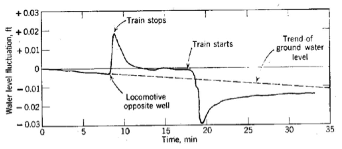
Fig. 5.10 Water level fluctuation in a confined aquifer produced by a train stopping near an observation well (Todd 1959; Todd and Mays 2005)
A nice and famous early example of loading efficiency is the impact of a train stopping at a station and leaving again some time later (Fig. 5.10). The weight of the locomotive compresses the aquifer a bit, thus reducing its pore space. This in turn compresses the groundwater, which cannot readily escape. Hence, its pressure rises and it starts to flow sidewards, so that the pressure gradually decreases towards its original trend. When the train leaves, the opposite occurs. The removal of the load reduces the effective stress, which causes the aquifer to bounce back, providing more pore space to the water, which depressurizes and increases somewhat in volume. This reduced water pressure causes surrounding groundwater to flow inward to fill up the gap due to which the pressure gradually normalizes.
Q: Think of another way for the water to escape from a semi-confined aquifer.
5.2.3. Barometer efficiency
Fig. 5.11 left shows the situation where the pressure increase is caused by a load (of sand) on ground surface; the right-hand picture shows how the same pressure increase is caused by an increase of the barometer pressure. The question is, how does the change of the barometer pressure alter the head (water level) in the piezometer?

Fig. 5.11 Effect on head in confined aquifer by a load \(\Delta p\) on surface versus an increase of the barometric pressure.
As said above, for the pressure in the aquifer there is no difference between the two pictures. However, there is a difference between the head (i.e. the water level) in the piezometer in the left picture and in that of the right picture. When placing a layer of sand on ground surface, the pressure on the water surface in the piezometer does not change. However, when the the barometer pressure changes, the pressure on the water surface in the piezometer does change. That change is, of course, exactly equal to the change of the barometer pressure. To see how the head changes due to a change of the barometer pressure let us just write out the water pressure at the bottom of the piezometer. It is clear that this pressure changes due to the change at ground surface such that \(\Delta a=\Delta p\), with \(\Delta a\) the change of the barometer pressure.
Now assume that the head (i.e. the water level) in the piezometer changes by an amount \(\Delta\phi\). The change of the water pressure at the bottom of the piezometer then is
But we already know the change of the water pressure
Hence,
and so
where \(1-LE\) is called the barometer efficiency, \(BE\). Just like the loading efficiency, the barometer efficiency varies between 0 and 1.
The minus sign indicates that the head in the piezometer declines when the barometer goes up. This should be obvious as the the water pressure increases by \(LE\,\Delta a\) which is a fraction of the barometer pressure, which would cause the water level in the piezometer to rise, but at the same time the full barometer pressure pushes on the water table in the piezometer, which causes the water level to decline accordingly. Together, the net effect is a decline of the head in the piezometer by \(BE\,\Delta a\), a fraction of the barometer pressure change.
From the equivalence of the previous equation couple, it follows that
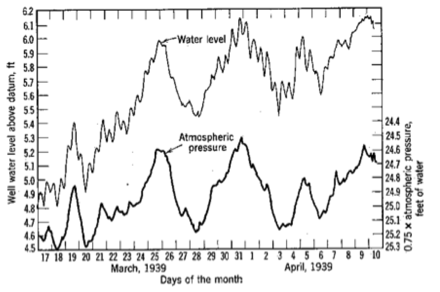
Fig. 5.12 Example of a high degree (75%) of barometric efficiency (Todd 1959; Todd and Mays 2005). It shows the response of the head in a well penetrating a confined aquifer together with the barometric pressure. Note that the axes on the right is reversed to show the similarity of the two curves (head down when barometer pressure goes up and vice versa).
A famous example of the barometer efficiency was given by (Todd 1959; Todd and Mays 2005), Fig. 5.12. This example is used here because it is famous as one of the first-ever published. However, barometer effects are always seen in piezometers in confined aquifers. The barometer efficiency generally varies between 20% and 80%.
The barometer influence causes a normally observed noisy behavior of the head time series from confined and semi-confined aquifers. This noisy behavior occurs also when groundwater is in perfect rest. Barometer pressure fluctuations do affect both the head measured in piezometers as the pressure measured in pressure gauges. Only if heads are measured at short time intervals of hours rather than weeks, would the noisy behavior of the head in confined aquifers actually show its clear one-to-one relation with the course of the barometer pressure. Therefore, such a noisy time series behavior actually shows that a piezometer is in a (semi-)confined aquifer. Unless we have very thick unsaturated zones with substantial resistance against air flow, we will not see much if any barometer fluctuation in water-table aquifers (Rasmussen and Crawford 1997).
5.2.4. How much are the loading efficiency and the barometer efficiency when expressed in the properties of the water and the porous medium ?
If the total pressure \(p\) is increased by \(\Delta p\), the porous medium is compressed together with the water that it contains. Clearly, the increase of the water pressure will also compress the individual grains. However, sand grains are about 50 times less compressible than water. Therefore, the effect of the grains being compressed themselves can be safely neglected.
On the other hand, the porous medium (the skeleton of grains) itself is far less stiff than the grains themselves. The porous medium is essentially compressed due to some deformation of the grains at the expense of the porosity of the medium. In fact, as it turns out, the compressibility of the porous medium is of the same order of magnitude as that of the water, so they must both be taken into account.
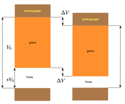
Fig. 5.13 Compression of the porous medium, while the volume of the grains remains unchanged because their compressibility is negligible compared to that of both the water and the porous medium.
Hence, the volume \(V_{0}\) is compressed by \(\Delta V\) when the pressure \(p\) is increased by \(\Delta p\).
Assume the aquifer to be of infinite lateral extent, so that the only possible compression is downward. This implies that \(\Delta V=\Delta H\), which is the change of the thickness of the considered part of the layer that we replaced by the springs in Fig. 5.9. Hence, both springs underlie the same compression \(\Delta H\).
Let the water have a compressibility \(\alpha\) meaning that a \(m^{3}\) of water would be compressed by the fraction \(\alpha\) for each increase of the water pressure by \(1\,\mathrm{N/m^{2}}\). Similarly, let the porous medium have a compressibility of \(\beta,\) meaning that one \(m^{3}\) of the porous medium would be compressed by the factor \(\beta\) for each \(\mathrm{N/m^{2}}\) increase of effective stress, \(\sigma_{e}\). These compressibilities, therefore, have dimension \(\mathrm{m^{3}/m^{3}/\left(N/m^{2}\right)}=\mathrm{m^{2}/N}\).
Now consider that the soil was put under an extra total pressure of \(\Delta p\) causing it to be compressed by the fraction \(\Delta H/H_{0}=\Delta V/V_{0}\). Then the effective pressure increases due to this compression \(\Delta H\) by
Because the grains are considered incompressible, it follows that the change of pore volume equals the change of the total volume. Therefore, for the water we have a relative volume change (= compression) of \(\Delta V\) per \(\epsilon V_{0}\). Therefore, the water pressure increase is
Because we have now related both \(\Delta\sigma_{w}\) and \(\Delta\sigma_{w}\) to the relative volume change \(\Delta V/V_{0}\), we also know the ratio between the change of the effective pressure and the water pressure
and so
With this, we can eliminate \(\Delta\sigma_{e}\) from the pressure equation:
to obtain
And because \(\Delta\sigma_{w}/\Delta p=LE\) we have
And because \(BE=1-LE\) we also have
5.2.5. Specific (elastic) storage coefficient
The specific storage coefficient is the change of volume per unit volume of space per unit change of head:
it is the volume of water released from the porous medium per m of lowering of the head \(\phi\) (a negative \(\Delta\phi\) yields a positive amount of water). It is also immediately clear that the dimension of \(S_{s}\) is \(\mathrm{\left[m^{3}/m^{3}\right]/m=m^{-1}}\), the volume of water released per \(\mbox{m}^{3}\) of the porous medium per m of head decline.
Now consider the situation in which we lower the water pressure, for instance by extracting water from the aquifer. Lowering of the water pressure in no way changes the total pressure. Therefore, \(\Delta p=0\), which yields
However, the amount of water squeezed out of the porous medium changes. A lowering of head causes an increase of the effective pressure (grain pressure), and, hence, is associated with a compression of the porous medium. Therefore, an increase of the effective pressure ( \(\Delta\sigma_{e}>0\)), reduces the pore volume by \(\Delta V\) due to which the same volume of water is squeezed from the porous medium
where \(pm\) means ”porous medium ”.
An increase of the water pressure, would cause a compression of the water within the pores \(\epsilon V_{0}\), by
The total amount of water released equals the volume squeezed out due to the reduction of the pore space plus the volume that is generated by expansion of the water due to the reduction of the water pressure:
and because \(\Delta\sigma_{e}=-\Delta\sigma_{w}\) in this case (see (5.3)), we have
so that
now with \(\Delta\sigma_{w}=\rho g\Delta\phi\) get 4.14
and, therefore
so that with \(S_{s}=-\frac{\Delta V/V_{0}}{\Delta\phi}\), we now have a formula that allows us to compute the specific elastic storage coefficient to the physical elastic properties of the aquifer, \(\beta\), and the water, \(\alpha\).
which, considering that we reduce the \(\Delta\) to the infinitesimally small \(\partial\), completes the proof (see (5.2)).
Notice the dimension of \(S\)
As often is more practical to write the dimension of gravity \(g\) as \(\mathrm{\left[\frac{N}{kg}\right]}\) instead of \(\mathrm{\left[\frac{m}{s^{2}}\right]}\). They are the same, the first can be seen as the force in \(N\) by which gravity pulls a mass of 1 kg downward; the second as the acceleration a mass of 1 kg would undergo when freely left to gravity to fall.
5.2.6. Application (not for exam)
The compressibility of water is
where \(\alpha\approx4.4\times10^{10}\,\mathrm{m^{2}/N}\). Clearly, \(\partial V_{w}/V_{w,0}\) is the relative change of the water volume. There is some dependency on dissolved components, water containing dissolved gas, may be up to three times more compressible than water without dissolved gas under normal pore pressure (Lyons, William C. (2010): Working Guide to Reservoir Engineering; Elsevier).
The compressibility of the porous medium is
where \(\partial V_{T}/V_{T,0}\) is the relative change of the volume of the porous medium. \(V_{T}\) is, the total volume of the considered soil (including its pores). \(\sigma_{e}\) is the effective stress (=grain pressure), i.e. that part of the total stress, \(p\), that is not carried by the water pressure \(\sigma_{w}\). The total pressure equals the weight of the overburden, i.e. that of the overlying formations including the water that they contain. Hence \(\sigma_{e}=p-\sigma_{w}\).
The soil compressibility \(\beta\) is the gradient of a stress-strain curve (relative volume change as a function of effective stress) of a dry soil sample put under increased stress in the laboratory, such that side-ward movement is prevented, exactly as it is the case in the actual aquifer under uniform vertical stress. Unlike water, the compressibility of soil is not necessarily a constant. If the soil is put under higher stress than it had ever supported before, then it consolidates, meaning that the change of volume is largely irreversible. But under lower than historic stresses, a constant compressibility can be determined, and truly elastic behavior can be assumed. It should be clear, that this compressibility depends on porosity.
Gun (1980) presented the following relationship between the compressibility of aquifers and depth based on laboratory measurements that were carried out by Van der Knaap (1959, unfortunately no direct reference).
where \(z\) in [km] is the depth below ground surface and \(\epsilon\) is porosity. Then we can apply (5.5)
With the relation of Gun (1980), we obtain the graphs shown in Fig. 5.14. As can be concluded from the graph, values in the order of \(10^{-5}\,\mathrm{Pa^{-1}}\) are often found in practice, where we generally have porosities of around 35% in fluviatile and eolian sandy aquifers.
Question: Is it feasible that compressibility of the porous medium is proportional to porosity?
![Computed specific storage coefficient :math:`Ss=\rho g\left(\epsilon\alpha+\beta\right)\,\mathrm{\left[m^{-1}\right]}` as a function of depth below ground surface using the relation by Gun (1980).](_images/SsVdGun1980.png)
Fig. 5.14 Computed specific storage coefficient \(Ss=\rho g\left(\epsilon\alpha+\beta\right)\,\mathrm{\left[m^{-1}\right]}\) as a function of depth below ground surface using the relation by Gun (1980).
5.2.7. Questions
Explain what loading efficiency is.
What factors contribute to the elastic storage coefficient and what factor may be neglected?
If a load \(\Delta p\) is placed on top of a confined aquifer and the water pressure in the aquifer is increased to \(\Delta\sigma_{w}=LE\,\Delta p\), then how much does the head change in a piezometer in that aquifer?
The same question for the situation where \(\Delta p\) is caused by an increase of the barometer pressure.
Assume we have a pressure gauge (often also called pressure transducer or pressure sensor) in a piezometer in the confined aquifer that measures the absolute pressure (i.e. the atmospheric pressure + the water pressure). On day 1, the barometer rises by \(\Delta p\) and is constant thereafter. Later, a load \(\Delta p\) is placed on ground surface. What is the difference, if any, in the registration done by the pressure gauge in the piezometer, and what is the difference with the hand-measured head in the piezometer?
The measurements by pressure gauges in confined and semi-confined aquifers are corrected for barometer pressure changes by subtracting the barometer pressure from the measured pressure. Does this mean that the fluctuations of the barometer pressure are eliminated by this correction? If so, explain why. If not, also explain why.
What is actually the result of this correction of the registered pressures? What actually do we get by this correction?
- How can we compute the specific elastic storage coefficient \(S_{s}\) from the measured barometric efficiency? Note:\[\begin{split}\begin{aligned} BE & = & 1-\frac{\beta}{\epsilon\alpha+\beta}\\ Sy & = & \rho g\left(\epsilon\alpha+\beta\right)\end{aligned}\end{split}\]
Think of what we can easily estimate and what we know, respectively what we don’t know? Assume that porosity \(\epsilon\) can be reasonably well estimated.
Consider a confined aquifer and the following two situations. First there is a loading at ground surface with value \(\Delta p\). The head is measured both in a piezometer and in a pressure gauge (which measures the absolute water pressure in the aquifer). What is the difference between the two measurements?
In the same location, consider an increase of the barometer pressure that is of the same magnitude as the surface loading \(\Delta p\) before, so \(\Delta a=\Delta p\). What is the difference in the head measured with a piezometer and that measured with a pressure gauge?
What is the difference between the heads measured with the piezometer in the two cases?
What is the difference between the pressures measured with the pressure gauges in the two cases?
How much is the barometer effect in an unconfined aquifer?
How will the head or pressure in a piezometer in a semi-confined aquifer after a uniform surface load was put on the ground surface? Think of compression and leakage through the overlying aquitard.
What aquifer parameter might we derive from this behavior? Think of the leakage.
With two pressure transducers, one measuring the barometer pressure and the other the water pressure in some piezometer in a confined aquifer, how can we compute the barometer efficiency? What parameter do we still miss to obtain true numerical values?
How does the head in a water-table aquifer react to barometer fluctuations?
How large may the variation of the head due to barometer fluctuations become given a range of atmospheric pressure from variation between 970 to 1040 mbar (=cm head)?
What values do you expect for total elastic storage coefficients of aquifers in practice?
How could we measure the elastic storage coefficient in a confined aquifer below the sea bottom?
Does the value of the specific yield that we may derive from barometer efficiency, water storativity and porosity refer to the value of the measuring point or to the thickness of the entire aquifer?
How useful is it to measure local porosity at the screen position of the piezometer to compute the storage coefficient of the aquifer?
5.3. Earth tides (not for exam)
Even far from the ocean and even after correcting for varying barometer pressures, the groundwater head in confined aquifers may show a response that closely resembles tides. This fluctuation matches the passage of the sun and the moon due to a rotating earth, exactly like it is the case with sea tides, ((Todd 1959; Todd and Mays 2005; Boemen, Lekkerkerker, and Molen 1989)), Fig. 5.15.
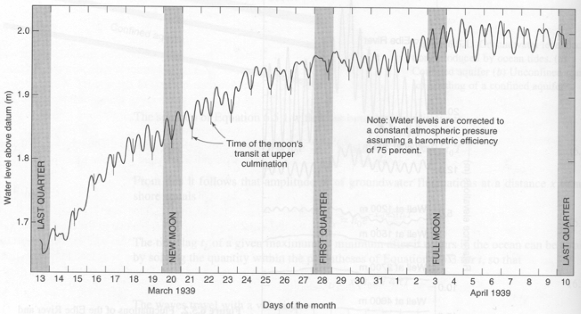
Fig. 5.15 Water level fluctuations in a confined aquifer produced by earth tides (from Todd (1959; Todd and Mays 2005))
Like normal tides, earth tides are an indirect consequence such gravity variations. It can be shown that they are caused as an indirect effect of the deformation of the earth’s mantle on which the stiff crust floats. A bulge is formed by the mantle by the attraction of the sun and the moon. The earth crust itself is so thin compared to the earth mantle that it behaves like a thin hard sheet floating on the mantle and is stretched by the mantle as it bulges out under tidal attraction. During stretching, porosity increases and the head lowers. When the stretching is released, the opposite occurs as is shown in Fig. 5.15.
This variation may be estimated with up to 50% accuracy from solid earth-tide theory (Kamp and Gale 1983). The dilatation (stretching) is more or less fixed due to the relation with the mantle, but different, for any point on earth. According to Bredehoeft (1967) it is about
at moderate latitudes. Using this number, one may relate the expected magnitude of the water-level fluctuations directly to the specific storage coefficient. With \(S_{s}\) in the order of \(10^{-6}\)/m for sandstones and \(10^{-7}\)/m for granites, a fluctuation amplitude of 1 to 10 cm may be expected.
A thorough analysis of earth tides is beyond the scope of this course. There is a wealth of literature on the subject; a good quantitative paper is Kamp and Gale (1983).
6. One-dimensional transient groundwater flow
6.1. Scope
In this course, we will deal with transient groundwater flow in one-dimensional and radial situations (wells) for which analytic solutions are available. Analytic solutions are important because they allow insight in the behavior of the groundwater system, whereas numerical solutions do not; they only produce numbers. Analytic solutions are also important because they allow checking numerical models and checking numerical models is always necessary, not just because of possible errors in the model, but also because of possible errors in the input of the model. Analytical solutions also allow analysis of numerical models, which helps to understand their outcome. Finally, analytical solutions are powerful because they allow a rapid result with minimal input. They become even more powerful if combined with superposition and convolution.
6.2. Governing equations
We will always start our discussion with the governing differential equation at hand. Once we have it, we need to solve it. To be able to do that we need boundary conditions specifying fixed heads or fixed discharges along certain parts of the model boundaries. In the case of transient solutions, we also need initial conditions that specify the head everywhere in the considered domain at time zero. Initial and boundary conditions are as important as the differential equation itself.
One-dimensional flow means a cross section with no-flow components perpendicular to it.
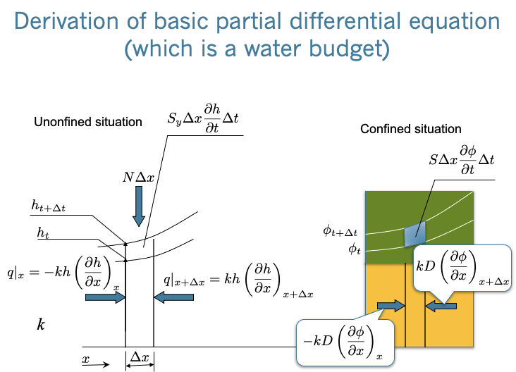
Fig. 6.1 Derivation of basic partial differential equation (left an unconfined aquifer with \(h\) the water-table elevation and \(S_{y}\) specific yield, and right a confined aquifer with \(\phi\) head, \(S\) elastic storage coefficient)
We will treat analytical solutions for one layer only. Analytical solutions for more than one layer exist and have been extended to arbitrary numbers of layers in the 1980s by Kick Hemker and Kees Maas, see for instance Hemker (1985; Maas 1986; Hemker and Maas 1987). These solutions require matrix computations, which were cumbersome at the time, but which may nowadays be readily computed in programs like Python. Nevertheless, we limit ourselves in this course to single-layer cases.
Let us first derive the partial differential equation, starting with continuity. Considering a small slice of an aquifer of length \(\Delta x\) (cross section) and write its dynamic water budget in terms of flow rates, assuming a constant aquifer thickness \(D\)
Dividing by \(\Delta x\) and by \(kD\) (assumed constant) yields
Letting \(\Delta x\rightarrow dx\) yields
We ignore the recharge \(N\) in this course, as we can always superimpose its effect so that with \(N=0\) we get
Further notice that we may write \(s\left(x,t\right)=h\left(x,t\right)-h_{0}\) where \(s\left(x,t\right)\) is the head change relative to the initial situation \(h_{0}\), which may even depend on \(x\).
Also notice that often \(h\) is used for the head in a water table aquifer, i.e. the elevation of the water table and \(\phi\) for the head in a confined or semi-confined aquifer, i.e. where there is not water table. In fact, it matters little what symbol is used, as long at its meaning is clearly stated.
This means that for 1D groundwater dynamics, we will mostly work with solutions of the following partial differential equation where \(s=s\left(x,t\right)\) is called the head change or often also the drawdown, especially when dealing with groundwater extraction and wells
(6.2) is known as the diffusion equation. It appears in many scientific fields like like diffusion, dispersion, heat conduction, sorption, consolidation, etc. Many researchers have derived solutions for this partial differential equation for specific boundary and initial conditions. The coefficient \(S/kD\) is called the diffusivity, often written as a thick D, like \(\mathbb{D}\), which always has dimension \(\mathrm{\left[L^{2}/T\right]}\) whatever the scientific application is. The diffusivity is the ratio of the ease of the flow (transmissivity) and the storage:
In the case of a phreatic (unconfined, water-table) aquifer, the aquifer thickness is no longer constant. Unfortunately, there are no transient solutions that take a time-varying aquifer thickness into account. Linearization is then unavoidable, meaning that one has to choose a proper average aquifer thickness (or transmissivity) and remain vigilant that the head change should remain small with respect to the saturated thickness of the aquifer.
The partial differential equation can also be viewed in this basic left-hand and right-hand parts
in which the left-hand side describes the flow in the aquifer and the right-hand side the storage. To readily understand and let sink in the meaning of this partial differential equation, it is perhaps easiest to integrate both sides over a distance \(\Delta x\) to get
which equals
This clearly shows that the left-hand side is the net inflow of a piece with length \(\Delta x\) (having dimension [L \(^{2}\)/T] or [L \(^{3}\)/T] per unit length perpendicular to the cross section of the aquifer, hence [L \(^{2}\)/T], while the right-hand side equals the storage over the same aquifer distance with \(S\) [L \(^{3}\)/L \(^{2}\)/L] (volume per unit of aquifer surface area per unit of head increase per unit of time).
Also notice that
is the curvature of the head. Whenever that is positive, there is an net inflow at the considered location originating from the aquifer adjacent to the considered point or infinitesimally small section.
Finally notice that we can replace the head change \(s\) (normally used for (semi-)confined aquifers) by the absolute head \(h\) (normally used for water-table aquifers). This makes absolutely no difference as only the derivatives of \(s\) and \(h\) play a role in the equation, which are the same. Just read \(s\) as head difference relative to some initial or average condition.
6.3. Sinusoidal fluctuations of the groundwater head and flows
This section deals exclusively with sinusoidal fluctuations of groundwater heads and flows caused by a head of flow that fluctuates like a sine at \(x=0\). We deal with tidal fluctuations in groundwater first and then show temperature as a second application of the same basic partial differential equation.

Fig. 6.2 Sinusoidal water level fluctuation in surface water causing tide in the groundwater system
6.3.1. Groundwater fluctuations due to sinusoidal tides
A number of transient problems can be analyzed by assuming sinusoidal water-level or flow fluctuations at a boundary, at \(x=0\) say. Generally, the resulting heads and flows within the aquifer will then also behave like a sine which will have the same frequency. If we have the analytic solution for head or flow in the aquifer due to harmonic fluctuating at the boundary, we may solve many related and more complex problems by superposition, that is by combining solutions of arbitrary frequencies, amplitudes and phase shifts. This way, hourly, daily, weekly and seasonal fluctuations may be readily combined. Examples of applications are tides in groundwater en the depth penetration of temperature fluctuations at ground surface.
Fig. 6.2 shows a cross section through a confined aquifer (yellow) that extends to infinity at the right. At \(x=0\) this aquifer is in direct connection with a surface-water body with a fluctuating water level, which causes fluctuations of head and flow in the adjacent aquifer, which are delayed and dampened relative to the forced fluctuation at \(x=0\).
The partial differential equation for this system has already been derived (see (6.2)). It may be solved for a sinusoidal fluctuation of the water level at \(x=0\). We just assume the solution of the head \(s\) in the aquifer relative to the mean value without fluctuation, to be also sinusoidal with the same frequency (same angular velocity \(\omega\) [radians/T]), but add a phase shift ( \(-bx\)) and assume an amplitude which is reduced by the factor \(e^{-ax}\) relative to the amplitude \(A\) of the tide at \(x=0\):
The full tide time \(T\) relates to the angular velocity \(\omega\) as
Notice that we can always change the phase of the tide by adding an arbitrary angle \(\nu\) to the argument of the sine. For an aquifer with constant \(kD\) and storage coefficient \(S\) this solution is indeed valid for
The proof is given in the box below. The proof fills the presumed solution into the partial differential equation and sees under which conditions the solution is true. It turns out to be as given in (6.5). The relations may also be derived for the situation in which the aquifer is semi-confined. Of course, this is more complicated and beyond this course. However, the solution is given in the box below for possible future reference.
Below the proof is given for the solution
As can be seen, an the arbitrary constant \(\beta_{0}\) does not affect the proof of correctness. This constant is merely a phase shift at \(t=0\). Therefore, the solution can also be given including this extra phase shift at \(t=0\), which may be useful when superimposing many fluctuations that differ in amplitude was well as in phase:
To see that \(\beta_{0}\) is a phase shift, just fill in \(x=0\) and \(t=0\).
The discharge is obtained by using Darcy
Hence, phase the flow is shifted by \(\pi/4\) relative to the head.
As an example, Fig. 6.3 upper image shows the head as a function of \(x\) for different times and the lower image shows the head as a function of \(t\) at different distances from the boundary. The upper figure also shows the upper and lower envelopes, although a bit difficult to see. The third picture is the discharge as a function of time at different \(x\)-values. The head in the second picture reaches its top when the discharge at the considered point is already declining.
![First picture: head as a function of :math:`x` at different times, also showing the upper and lower envelopes. Second picture: head as a function of t at different distances. :math:`A=1.5` m, :math:`kD=600` m\ :math:`^{2}`/d, :math:`S=0.001`, :math:`\omega=4\pi` (i.e. two full tide cycles in 1 D). Third picture, discharge :math:`Q` [m\ :math:`^{2}`/d] (to the right positive) as a function of time for different :math:`x`-values.](_images/sines_f_x.png)
Fig. 6.3 First picture: head as a function of \(x\) at different times, also showing the upper and lower envelopes. Second picture: head as a function of t at different distances. \(A=1.5\) m, \(kD=600\) m\(^{2}\)/d, \(S=0.001\), \(\omega=4\pi\) (i.e. two full tide cycles in 1 D). Third picture, discharge \(Q\) [m\(^{2}\)/d] (to the right positive) as a function of time for different \(x\)-values.
![First picture: head as a function of :math:`x` at different times, also showing the upper and lower envelopes. Second picture: head as a function of t at different distances. :math:`A=1.5` m, :math:`kD=600` m\ :math:`^{2}`/d, :math:`S=0.001`, :math:`\omega=4\pi` (i.e. two full tide cycles in 1 D). Third picture, discharge :math:`Q` [m\ :math:`^{2}`/d] (to the right positive) as a function of time for different :math:`x`-values.](_images/sines_f_t.png)
Fig. 6.4 First picture: head as a function of \(x\) at different times, also showing the upper and lower envelopes. Second picture: head as a function of t at different distances. \(A=1.5\) m, \(kD=600\) m\(^{2}\)/d, \(S=0.001\), \(\omega=4\pi\) (i.e. two full tide cycles in 1 D). Third picture, discharge \(Q\) [m\(^{2}\)/d] (to the right positive) as a function of time for different \(x\)-values.
![First picture: head as a function of :math:`x` at different times, also showing the upper and lower envelopes. Second picture: head as a function of t at different distances. :math:`A=1.5` m, :math:`kD=600` m\ :math:`^{2}`/d, :math:`S=0.001`, :math:`\omega=4\pi` (i.e. two full tide cycles in 1 D). Third picture, discharge :math:`Q` [m\ :math:`^{2}`/d] (to the right positive) as a function of time for different :math:`x`-values.](_images/sindes_Q_vs_t.png)
Fig. 6.5 First picture: head as a function of \(x\) at different times, also showing the upper and lower envelopes. Second picture: head as a function of t at different distances. \(A=1.5\) m, \(kD=600\) m\(^{2}\)/d, \(S=0.001\), \(\omega=4\pi\) (i.e. two full tide cycles in 1 D). Third picture, discharge \(Q\) [m\(^{2}\)/d] (to the right positive) as a function of time for different \(x\)-values.
6.3.1.1. What is the velocity of the wave, or what is the delay of the wave at any distance \(x\) from the sea or river?
To find the answer, we move along with the wave such that the phase is constant, e.a. equal to \(c\). Hence
Then determine the velocity by computing \(dx/dt\). So
This leads to
The delay of the wave at any \(x\) relative to the wave at \(x=0\) is then
The wave velocity can be measured in Fig. 6.3 as the velocity of the top of the sines in the third figure .
Alternatively, one may say, that when the argument must be constant, it doesn’t matter which constant, but only constant, then we can just well say that
so that immediately we have \(x/t=\omega/a\), which is the same answer.
6.3.1.2. How much is the wavelength in the ground?
A direct approach is taking the argument of the sinus and demanding that the argument of the sine at \(t+T\) at \(x\) (where \(T\) is the cycle time) is the same as the argument of the sine at \(t\) but at location \(x+\Delta x\)
hence
noting that the cycle time equals \(T=\frac{2\pi}{\omega}\), we get
with \(a=\sqrt{\frac{\omega S}{2kD}}\), we also have
So, the larger \(kD\) the longer the wave length, the larger the \(S\) the shorter and the larger the \(\omega\), the shorter the wavelength will be, which all makes sense.
We have now seen that the head is indeed a damped sine. The damping is stronger for higher frequencies, larger storage coefficients and lower conductivities. It’s difficult to measure the wave length from the upper figure in Fig. 6.3 because the damping is so strong that essentially full damping takes place within a single wavelength.
6.3.2. Using characteristic time and length
The solution may be more intuitively expressed using characteristic time and length. The charactersitci time would be the cycle time, \(T\), i.e. it takes for one full tide to complete
Also, we could set a characteristic length of the tide the aquifer to
The envelopes are thus now expressed as
so that \(\lambda\) now is the length over which the maximum amplitude declines by a factor \(e\approx2.3\).
The relation with the length over which the amplitude declines by exactly a factor 2 is easily derived
As always when we have an exponentially declining relationship, we can define a half-time or half-length. That halftime or half-length is always \(\ln\left(2\right)\approx69\%\) of the characteristic time of characteristic length, i.e. the time or length in which the exponent declines by a factor \(e\approx2.3\).
The characteristic length of the tidal wave in the aquifer is, therefore
and the half-length is just 69% of this.
Filling in the characteristic length and time gives
If one wishes to express all terms within the argument of the \(\sin\) in terms of the full tidal cycle, one would write
This directly shows that the distance \(x=2\pi\lambda\) is the length of a full wave in the subsurface, and, therefore, the expression \(2\pi\lambda/T\) is the velocity of the wave in the subsurface.
which is, what we already derived in What is the velocity of the wave, or what is the delay of the wave at any distance x from the sea or river? . This all seems needlessly complicated, but the take-home message is, that thinking in terms of cycle time and characteristic length is easier for the human mind and can be immediately translated to the field situation, while \(\omega\) and the damping and delay factor \(a\) really provide far little inspiration.
6.3.3. Fluctuations of temperature in the subsurface
For heat conduction in the subsurface, the same partial differential equation (also called“diffusion equation”) applies if we replace head change by temperature change. The only thing that changes is the so-called diffusivity \(kD/S\). The ease of flow, i.e. \(kD\) with groundwater flow, is now replaced by the heat conduction \(\lambda\,\mathrm{\left[W/m\right]=\left[\left(\left(E/T\right)/L^{2}\right)/\left(K/L\right)\right]=\left[E/\left(TKL\right)\right]}\) and the storage is replaced by the heat capacity \(\rho c\,\mathrm{\left[E/L^{3}/K\right]}\). The dimension is again \(\mathrm{\left[L^{2}/T\right]}\):
Notice that in the dimension \(E\) = energy, \(T\) = time, \(L\) = length, \(K\) = temperature (from Kelvin). Because both the heat conduction and the heat capacity consist of a contribution from both the water and the grains (solids) of the aquifer, we can compute them as a porosity-weighted combination of these contributions. With \(\epsilon\) for porosity we then have
\(\rho\,\mathrm{\left[M/L^{3}\right]}\) is density and \(c\,\mathrm{\left[E/\left(MK\right)\right]}\), i.e. heat per kg solids per degree kelvin (= degree Celsius).
The heat capacity of saturated sandy soils is about \(\lambda=3\,\mathrm{W/m/K}=3\,\mathrm{J/s/m/K}\). The specific heat capacity of water is \(c_{w}=4018\,\mathrm{J/kg/K}\) and that of sand grains \(c_{s}\approx800\,\mathrm{J/kg/K}\). With \(\rho_{s}\approx2650\,\mathrm{kg/m^{3}}\) and \(\epsilon\approx35\%\) we get \(\rho c=2.85\times10^{6}\,\mathrm{J/m^{3}/K}\).
The diffusivity then becomes
From which we have
With these values, one can compute between what values the temperature varies at any given depth as a function of the cycle time. For instance, the temperature fluctuation due to daily, weekly, monthly or yearly temperature fluctuations at ground surface. These envelopes are defined by
with \(A\) [K] the temperature fluctuation amplitude at ground surface.
The monthly temperature in the Netherlands varies between 3.1 \(^{o}\)C in January and 17.9 \(^{o}\)C in July. The yearly amplitude is thus 7.4 \(^{o}\)C; the year mean temperature being 10.5 \(^{o}\)C. Using this, we can compute the temperature envelopes, that is, the lowest and highest temperatures between which the actual temperature will vary. Fig. 6.6 shows the results, as computed for the same mean temperature and the same amplitude but for different cycle times as indicated in the legend. With these data, the yearly temperature variation will barely reach 20 m below ground surface. Ten-year temperature fluctuations will penetrate down to about 50 m and 30 year temperature variation would be recordable down to about 100 m. This implies that climate change may be measured using the change of the temperature at for instance 50 m below ground surface if measurements in the past are available, as is actually the case in the Netherlands.
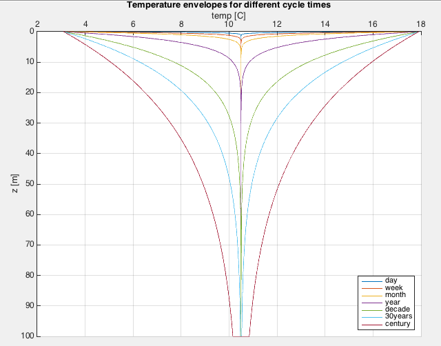
Fig. 6.6 Temperature envelopes in the subsurface due to temperature fluctuations at ground surface with mean 10 \(^{o}\)C and amplitude 7.4 \(^{o}\)C. Envelopes depend on cycle time of the fluctuation (see legend).
6.3.4. Concluding remarks
The derived partial differential equation applies to both groundwater flow and heat conduction. The only change is that head change is replaced by temperature change, transmissivity by heat conductance and the storage coefficient is replaced by heat capacity. Both heat conductance and heat capacity can be computed as a porosity weighted average of the contribution of the water and of the grains.
Sinusoidal analysis is useful to study the impact of ongoing fluctuations of the input on the groundwater. It is straightforward to compute the head and temperature envelopes defining the limits of a given sine input at a given distance or depth. Often, this is enough he understand the physics and estimate potential impact. Most importantly it is enough the understand the relation between the different parameters that play in this setting.
More complicated inputs can be constructed as a sum of a number of sin (or cosine) fluctuations, each with its own amplitude, frequency and phase shift. In fact, any input can be so constructed, although this may require the summation of many waves. On the other hand a given i.e. measured input may be split into individual waves using Fourier Analysis. Python has modules for that. This helps to find the dominant ones, and allows limiting the following analysis on only a few dominant waves. This simply means that this sinusoidal solution of the partial differential equations offers many ways to analyze groundwater systems of the type we considered. By superposition, these analysis can also be combined with other features such as wells.
6.3.5. Questions
Prove the correctness of the given solution yourself. As an extra exercise you could prove that (6.7) is correct by filling it into the partial differential equation for continuity \(\frac{\partial Q}{\partial x}=-kD\frac{\partial^{2}s}{\partial x^{2}}=-S\frac{\partial s}{\partial t}\).
If the transmissivity is doubled, what is the effect on the drawdown?
When the \(\omega\) is doubled, what is the effect on the drawdown?
Explain how the distance to where the fluctuation of the sea or lake reaches in the aquifer depends on the frequency of the wave.
How far in-land reaches the effect of waves on the beach with one cycle per second, tides with one cycle per 12 hours, moon-tides with one cycle per two weeks in an aquifer with transmissivity is \(kD=500\) m\(^{2}\)/d and a storage coefficient of \(S=0.001\) and \(S=0.1\) respectively?
Let the solution to the diffusion equation for the confined aquifer be \(s\left(x,t\right)=A\,\exp\left(-ax\right)\sin\left(\theta_{0}+\omega t-ax\right)\) and let \(kD=1000\,\mathrm{m^{2}/d},\) \(S=10^{-3}\), and the amplitude \(A=2\,\mathrm{m},\) and let \(\theta_{0}\) be an arbitrary constant. Take time in days and show the head change \(s\left(x,t\right)\) in Python or in Excel. With this, answer the following 5 sub-questions:
Include the discharge \(Q\left(x,t\right)\)
Compute and also show the envelope of the wave as a function of \(x\).
How far inland can we still measure the tide if our device allows us to see a variation of 1 cm?
What is the velocity of the wave?
What is the delay at 1000 m from the shore (or show the delay graphically as function of \(x\))?
Add the case for a storage coefficient, \(S_{y}=0.2\). And show the relation between the case with \(S=0.001\) and \(S_{y}=0.2\).
Create a complex input using of 4 sines, each with a different initial angle \(\theta_{0}\), amplitude \(A\) and angular velocity \(\omega\) and show the result.
Copy your code and alter the copy to answer the following questions:
The head in a lake above a clay bottom varies daily 30 cm. How deep does this fluctuation penetrate the underlying clay layer with conductivity of \(10^{-4}\) m/d and a specific storage coefficient of \(S_{s}=0.0001\) /m? Assume that you could still measure variations down to 3 mm.
What if the variation is weekly, monthly and seasonally only?
If the sea is shallow and the clay layer is below the sea bottom, what will be the amplitude in the confined aquifer for the water compressibility \(\beta_{w}=5\times10^{-5}\) and porous matrix compressibility \(\beta_{s}=2\times10^{-5}\,\mathrm{m^{2}}/N\)?
If the clay layer would be semi-pervious, what would this mean for the amplitude in the confined aquifer? Would it be greater, smaller compared with the case with a completely impervious layer?
6.3.5.1. Heat flow
What is the penetration depth of a diurnal (twice-a-day), seasonal and centennial temperature fluctuation at ground surface given \(\lambda=3\) W/m/K, \(\rho_{s}c_{s}=0.800\) MJ/m \(^{3}\)/K and \(\rho_{w}c_{w}=4.2\) MJ/m \(^{3}\)/K and porosity of \(\epsilon=0.35\)?
Heat flow and groundwater flow show the same partial differential equation except that head change is replaced by temperature change. They both have one coefficient called diffusivity. What is the dimension of this diffusivity in both situations?
Diffusivity consists of a part that expresses the ease of flow, \(\lambda\), and a part that expresses the storage, \(\rho c\). What are the equivalent factors in the groundwater case?
Groundwater flow was ignored when we discussed heat flow. Describe how temperature envelopes would change due to upward groundwater seepage, would they shrink or stretch?
How would these envelopes change due to downward seepage? How much would you estimate the effect on the yearly temperature envelopes if the recharge is 333 mm per year and porosity is 33%? First estimate how deep the recharge penetrates in one year.
6.4. Non-fluctuating interaction with surface water
In the previous section, we discussed the effect of sinusoidal variation of the level of a surface water that is in direct contact with a confined or unconfined aquifer. In this chapter, we’ll discuss the same hydrological setting, but in which the surface water level changes suddenly by a fixed amount.
6.4.1. Basins of half-infinite lateral extent
Again, we consider a confined aquifer in direct contact with surface water as was done in the previous section. The situation is depicted in Fig. 6.7. The aquifer thickness, transmissivity and storage coefficient are everywhere the same. The aquifer is half-infinite, which means that its right end extends to infinity. We consider the aquifer as confined, because we will assume that its thickness is the same everywhere and stays so. This is required only to allow a closed analytical solution for the time-dependent groundwater flow. There are no time-dependent closed analytical solutions for water-table aquifers in which the transmissivity varies along with the head and, therefore, with time. We further assume the aquifer being in direct contact with the surface water. This implies that there is no hydraulic resistance of any kind between the surface water and the aquifer. This assumption keeps the analysis simple. However, solutions exist that take hydraulic resistance between the surface water and the aquifer into account as outlined in Bruggeman (1999), but are beyond this course.
We present here a basic analytical solution, which describes the change of head (and flow) caused by a sudden change of the surface-water level by an amount \(A\) [m].
In the confined case we use the elastic storage coefficient, \(S=DS_{s}\) and in the unconfined case we use the specific yield, \(S_{y}\). In cases where we consider unconfined aquifers, the effective thickness of the aquifer changes along with the water table, and, therefore, also with the head. However, as long as the change of head is small compared to the thickness of the aquifer, we may still apply the solution in practice and accept the small error caused by the assumption of constant thickness.
Initially, the head is \(\phi'\) in Fig. 6.7 and the head \(\phi\left(x,t\right)\) varies in space and time due to a sudden change of head of the bounding surface water by an amount of \(A\) m at \(t=0\). The surface-water head remains at \(\phi'+A\) thereafter.
Because superposition applies (due to linear governing partial differential equation), we may just superimpose the change of head \(s\left(x,t\right)=\phi\left(x,t\right)-\phi'\), irrespective of the actual situation. The only thing that matters to us. is the change of head \(s\) that is caused by the sudden change of the water level in the bounding surface water by \(A\) m.
The case considered here is a base case. There exists a series of analytical solutions for other boundary conditions, which is presented in Higher-order solutions (not for exam). These solution are given for reference only, not for the exam.
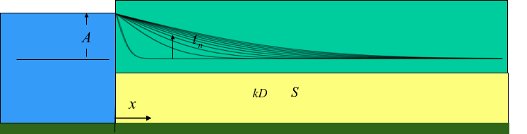
Fig. 6.7 One-dimensional groundwater aquifer which extends to infinity to the right, and has constant transmissivity \(kD\) and storage coefficient \(S\), while it is in direct contact with surface water at \(x=0\) in which the water level is suddenly changed by \(a\) at \(t=0\)
Consider a one-dimensional aquifer of infinity lateral extent as shown in Fig. 6.7 that is in direct contact with a fully penetrating water body at \(x=0\). Ignoring leakage and recharge, and assuming a constant transmissivity \(kD\) and storage coefficient \(S\), the partial differential equation is the diffusion equation:
The most well-known solution of this series of solutions is the one in which the head at \(x=0\) is suddenly raised at \(t=0\) by a \(A\) m, and then further maintained (figure 23).
This solution is
Where \(s\left(x,t\right)\) is the head change, \(\phi\left(x,t\right)\) the head and \(\phi_{0}\left(x\right)\) the initial head that may be any function if \(x\), because it does not interfere with the principle of superposition.
By definition
and so its derivative is
Therefore, the discharge is
and, for \(x=0\)
The function \(\mbox{erfc}(-)\) is the so-called complementary error function.
Abramowitz and Stegun (1972) provide tables and expressions to compute this function in several ways. The erfc function is available in Excel as well as in Python. Its graph is shown in Fig. 6.8
![[fig:Erfc(u)] :math:`\mbox{erfc}(u)` and its derivative :math:`-\left(2/\sqrt{\pi}\right)\exp\left(-u^{2}\right)`](_images/erfcFunction.png)
Fig. 6.8 [fig:Erfc(u)] \(\mbox{erfc}(u)\) and its derivative \(-\left(2/\sqrt{\pi}\right)\exp\left(-u^{2}\right)\)
![[fig:Erfc(u)] :math:`\mbox{erfc}(u)` and its derivative :math:`-\left(2/\sqrt{\pi}\right)\exp\left(-u^{2}\right)`](_images/erfcFunction_derivative_off.png)
Fig. 6.9 [fig:Erfc(u)] \(\mbox{erfc}(u)\) and its derivative \(-\left(2/\sqrt{\pi}\right)\exp\left(-u^{2}\right)\)
Hence, the solution of the head change versus distance to the shore always has the shape of this curve, be it that the horizontal axis will be squeezed or stretched depending on the values of the parameters in \(u\). The shorter the time, the larger \(u\), the more compressed is the horizontal axis. A small \(kD\) or large \(S\) also has the effect of compressing the horizontal axis.
For the understanding it is convenient to express \(u=x/L\) so that \(L=\sqrt{4kDt/S}\), which is a constant for any fixed \(t\). For this fixed \(t\), \(L\) may be considered a characteristic distance, as it scales \(x\). For instance, half of the initial head change has been reached when \(u\approx0.5\) that is at a distance \(x=0.5L\). Also, the head change is about 10% of \(A\) at \(u=1\), that is at \(x=L\), with \(L\) fixed for the time of observation. No head rise has yet occurred for about \(u=2.5\), hence, for \(x>2.5L\). This is all practical information when judging an actual situation, without the need for a computer.
The solution is only valid for \(u>0\), this is clear for \(x^{2}\) under the square root and \(t>0\). But when we express \(u\) as \(u=x\sqrt{\frac{S}{4kDt}},\)this is not so obvious. However \(x\) is must be positive and seen as the distance from the point of consideration to the boundary with the head change. So in case this boundary as a coordinate \(x_{b}\) and our point of consideration is \(x_{0}\) we should use \(x=\left|x_{0}-x_{b}\right|\) in the formula of \(u\), hence, treat \(x\) as a distance, being always positive.
It is also possible to plot \(\mbox{erfc}\,u\) and its derivative versus \(1/u^{2}\). To make the graph meaningful, we have to use a logarithmic scale for \(1/u^{2}\) as is shown in Fig. 6.10. The time scale is then proportional to \(t\). We can write \(u^{2}=T/t\) with \(T=x^{2}S/\left(4kD\right)\), where \(T\) can be considered a characteristic time for fixed distance \(x\). We see that for \(t/T\approx2\), about half the final (maximum) head change has been reached. It is useful and practical to consider this graph from the perspective of \(t/T\) instead of just \(t\). Taking this perspective, one only needs a single graph to cover all possible cases; the only thing that changes when choosing another observation point is the value of the characteristic time \(T\). Then \(T\) can be considered time characteristic for the situation at a chosen distance \(x\). The graph in Fig. 6.10 also shows that some time elapses before the influence of the river reaches the observation point. The value of \(1/u\) for this time is about 0.4 as can be read from Fig. 6.10. Hence, \(t/T=0.16\). This result is also universal. 90% of the final head is reached at about \(1/u^{2}=100\), so that \(t=100T\).
For the discharge, we need the derivative, which is also shown in both figures.

Fig. 6.10 erfc\(\left(u\right)\)and its derivative as a function of \(1/u^{2}\) instead of vs. \(u\). This makes the horizontal axis proportional to time, as \(1/u^{2}=\frac{4kD}{x^{2}S}t\).

Fig. 6.11 erfc\(\left(u\right)\)and its derivative as a function of \(1/u^{2}\) instead of vs. \(u\). This makes the horizontal axis proportional to time, as \(1/u^{2}=\frac{4kD}{x^{2}S}t\).
6.4.1.1. Exercise:
6.4.2. Questions
All drawdowns due to a sudden change of river stage are expressed in a simple erfc-function. Can you express the argument \(u\) using a ratio of the distance \(x\) from the river and some characteristic distance \(X\) that is valid for a fixed time?
What is the ratio \(x/X\) for \(s\left(x\right)=0.5s_{0}\), i.e. \(s\) is half the head change at \(x=0\)?
Alternatively, how could you express the head change as a ratio of time \(t\) and a characteristic time \(T\) for a fixed distance?
What is then the ratio \(t/T\) for \(s=0.5s_{0}\)?
At what time, expressed at \(t/T\), would you expect the head in the aquifer to start changing at some given fixed distance \(x\) after a sudden change of river stage at \(x=0\)?
Given the mathematical expression for the head change, derive the expression for the discharge \(Q\left(x,t\right)\).
What is the discharge at \(x=0\) mathematically?
An aquifer with properties \(kD=400\,\mathrm{m^{2}/d},\,S=0.1\) is in good contact with a river. The water level in the river rises by 2 m in a vary short time. What is the effect of this change for a points \(x\) at 10, 100 and 1000 m?
How long does it take for the head change in the three points to reach 10 cm?
Using Python, show the head over time in these points.
Using Python, show the discharge over time in these points.
How long will it take until the head in the center of a 10 m thick aquitard with resistance \(c=5000\) d and a specific storage coefficient \(S_{s}=10^{-5}\) m \(^{-1}\) has reached half the head change that was suddenly applied at both its top and bottom at \(t=0\)?
A canal in a dune area is used to provide storage for drinking water in the case of an emergency. The aquifer properties are \(kD=100\,\mathrm{m^{2}/d}\), \(S=0.2\). During such an emergency, the water level in the 50 m wide canal is suddenly lowered by 5 m.
How much water will flow into the storage canal from two sides in 1 day, 1 week, 6 weeks?
Compare these amounts with the amount of water stored in the canal?
What will be the drawdown over time at 10, 100, 300, 1000m?
Compute the flow to the canal in 6 weeks if there is a fixed-head boundary at 70 m distance. You must use superposition to compute this.
6.4.3. Higher-order solutions (not for exam)
The previous well-known basic solution is the first of an infinite series of solutions of the same partial differential equation but for different boundary conditions, namely \(s\left(0,t\right)=a\,t^{n/2}\) with \(a\) a constant and \(n\ge0\). The solution given above is for \(n=0\).
The entire series of solutions is given is given in Carslaw and Jaeger (1986) and Bruggeman (1999) but can be more conveniently written as
The function \(\mbox{i}^{n}\mbox{erfc}\,u\) is the \(n^{th}\) repeated integral of the complementary error function (Section 7.2 in Abramowitz and Stegun (1972)). A number of these functions is shown in Fig. 6.12. These higher order repeated integrals are not in Abramowitz and Stegun (1964) but can be easily computed using a recursive expression given below.
By definition
with
and
Higher order functions may be computed by the following recursive relation
By applying Darcy’s law, we find the discharge
Instead of expressing \(s\left(0,t\right)=At^{n/2}\) we could write \(Q\left(0,t\right)=Bt^{n/2}\), \(n\ge0\). This is more convenient when we like to specify the flow instead of the head. If we just write \(\frac{\sqrt{kDS}}{2\sqrt{t}}A=B\), we get
and at the same time
A basic solution is obtained by setting \(n=0\), so that \(Q\left(0,t\right)=B\) is constant. In that case, the head at \(x=0\) declines according to the \(\sqrt{t}\). When the discharge increases linearly, the head at \(x=0\) changes according to \(t\sqrt{t}\). On the other hand, when the drawdown is constant at \(x=0,\) the discharge is inversely proportional to \(\sqrt{t}\) and when the head at \(x=0\) rises linearly with time, the discharge increases according to \(\sqrt{t}\).
These functions may be used to compute the head and flow due to either a constant or changing head at \(x=0\) or due to a constant or changing flow at \(x=0\). Computations are easily done in Python or even in Excel after the functions have been implemented.
![[fig:-higher-order-erfc-functions] :math:`\mbox{i}^{n}\mbox{erfc}` functions](_images/ierfcFunctions.png)
Fig. 6.12 [fig:-higher-order-erfc-functions] \(\mbox{i}^{n}\mbox{erfc}\) functions
6.4.3.1. Example:
For instance, the water level in Lake Nasser in Egypt has risen by 60 m between the mid 1960s, when the dam at Aswan was closed, and the end of the 1980s, when the new lake was full. This boils down to rise of the lake level of about 3 m/year. Just assume that the bordering aquifer is 200 m thick and that it has a conductivity \(k=1\,\mathrm{m/d}\) and a specific yield \(S_{y}=0.1\). How far would the effect of the filling of the lake reach in the adjacent aquifer? How much lake water would have been stored in that aquifer in that same period?
Using the expression and setting \(n=2\) and \(A=3\) m/y, we have
This specifies a linear rise of the lake level over time. With \(n=2\) we get
With proper values of \(kD\) and \(S\), a graph can be made for \(s\) and \(Q\) as a function of \(x\) for given times. Alternatively, we can make graphs of \(s\) and \(Q\) as a function of time for given values of \(x\). The results are shown in Fig. 6.13. The top figure shows the head in the aquifer as a function of \(x\) for different times. The middle figure shows the infiltration at \(x=0\) as a function of time. The bottom figure shows the development of the head over time at different distances from the lake bank. Note that the lake level remains constant after \(t=20\) years. The head at \(x=0\), therefore, remains equal till the lake level reaches a total rise of 60 m thereafter. After that, the lake level is kept constant. The infiltration \(Q\) then sharply declines because the head does not rise further. This reaching of a constant lake level is implemented by superimposing the solution for a lake with a water level that declines with the same speed (i.e \(A=-3\) m/y) starting at the moment the top lake-level is reached. It is a good exercise to implement this yourself.
Of course, the same case can be simulated using the function for a sudden rise of the lake level. But then the actual gradual rise of the lake level must be subdivided into many small sudden steps, the result of which must be added together (i.e. superimposed) to obtain the overall solution. The results is shown in Fig. 6.16. The rise of the head and lake are shown in the lower picture, the flow at \(x=0\) is shown in the picture in the middle. The results are essentially the same, but the infiltration at \(x=0\) fluctuates quite heavily under the discrete yearly sudden head increments of 3 m each. At larger distances, however, these steps damp out. Of course, the smaller the steps, the smoother the result will be. This example shows that it may be much more convenient and require less work to directly apply the solution for the linear rise of the head at \(x=0\).

Fig. 6.13 Lake Nasser example. Top: the head in the adjacent aquifer as a function of \(x\), the distance to the shore, at different times. Middle: The infiltration into the aquifer at \(x=0\) as a function of time. Bottom: The head development over time at different values of \(x\)
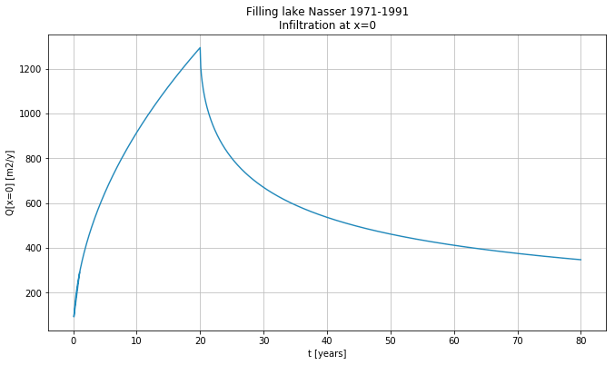
Fig. 6.14 Lake Nasser example. Top: the head in the adjacent aquifer as a function of \(x\), the distance to the shore, at different times. Middle: The infiltration into the aquifer at \(x=0\) as a function of time. Bottom: The head development over time at different values of \(x\)

Fig. 6.15 Lake Nasser example. Top: the head in the adjacent aquifer as a function of \(x\), the distance to the shore, at different times. Middle: The infiltration into the aquifer at \(x=0\) as a function of time. Bottom: The head development over time at different values of \(x\)
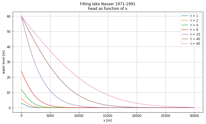
Fig. 6.16 Lake Nasser example, simulated using the solution for a sudden change and dividing the linear rise over 20 years in 20 sudden changes of equal size. Top: the head in the adjacent aquifer as a function of \(x\), the distance to the shore, at different times. Middle: The infiltration into the aquifer at \(x=0\) as a function of time. Bottom: The head development over time at different values of \(x\)

Fig. 6.17 Lake Nasser example, simulated using the solution for a sudden change and dividing the linear rise over 20 years in 20 sudden changes of equal size. Top: the head in the adjacent aquifer as a function of \(x\), the distance to the shore, at different times. Middle: The infiltration into the aquifer at \(x=0\) as a function of time. Bottom: The head development over time at different values of \(x\)

Fig. 6.18 Lake Nasser example, simulated using the solution for a sudden change and dividing the linear rise over 20 years in 20 sudden changes of equal size. Top: the head in the adjacent aquifer as a function of \(x\), the distance to the shore, at different times. Middle: The infiltration into the aquifer at \(x=0\) as a function of time. Bottom: The head development over time at different values of \(x\)
6.4.4. Questions
What is the mathematical expression for the head \(s\left(x,t\right)\) and the discharge \(Q\left(x,t\right)\) for the case in which the river stage increases linearly with time?
What is the mathematical expression for the case in which the discharge increases linearly with time.
Let a lake (like Lake Nasser) have a water level that rose linearly by 60 m between 1971 and 1991. Compute the change of head in the aquifer at 1 km from to the lake. Assume the \(kD=1000\,\mathrm{m^{2}/d}\) and \(S=0.1\).
Compute the total amount of water that infiltrated over this period.
Assume the aquifer has a constant thickness and its porosity is 35%. With this information compute how far the lake water penetrated the aquifer during this period.
When, after 1991, the water level has been more or less constant, then how much is the infiltration \(Q\left(0,t\right)\) at the lake shore in 2021? By how much has it declined since 1991?
6.4.5. Superposition in time, half-infinite aquifer
Consider a half-infinite aquifer in direct connection with surface water at \(x=0\). The analytical solution for the change of the groundwater head \(s\left(x,t\right)\) that is caused by a sudden change of the surface water level by an amount \(A\) at \(t=0\), which was given before :
The head change \(s\left(x,t\right)\) due to an arbitrary sudden change of the surface-water level by an amount \(A_{i}\) happening at \(t_{i}\) can be obtained by superposition as usual. Using \(i\) as an event index, we then get
Each term is nonexistent, hence zero, for \(t<t_{i}\). The surface-water level at any time is \(s\left(0,t\right)=\sum_{1}^{N}dA_{i}\mbox{, with }t>t_{ci}\), because each sudden change of water level is supposed to last forever after it happened at \(t_{ci}\). This way, one can compute the head change and, of course, the flow in an aquifer due to an arbitrary variation of the surface water level at \(x=0\). Of course, if the surface water would vary continuously, like one or more \(sine\) functions, one would rather use the solution for a sine boundary head to simplify the computations. Even a combination is possible, because superposition applies. Notice that the time \(t\) in the expression above is the simulation time and will be represented in the computer by an array of times at some arbitrary constant interval, while the time \(t_{ci}\) the“change”-time will be a series of times at which the surface-water level at \(x=0\) changes. The values \(t_{ci}\) are independent of the \(t\) values, and the number of change times is is usually much less than the number of \(t\) values.
We will simply compute the head due to the sudden head change \(dA_{i}\) happening at \(x=0\) at \(t_{ch_{i}}\) for all \(t>t_{ci}\) and add this to the head changes already computed for earlier times.
6.4.5.1. Example
Consider a situation with \(kD=400\,\mathrm{m^{2}/d}\) and \(S_{y}=0.1\). The river-water level \(A=\left[1.0,\,-0.5,\,+0.5,-0.25\right]\) at \(t_{c}=\left[0.5,\,0.8,\,1.0,\,2.0\right].\) Show the groundwater level as a function of time for \(x=50\) m for \(0\le t\le5\) d. In this case it is convenient to take \(t\) in hours to get sufficient detail.
Fig. 6.19 gives the results for \(x=100\) m as a function of time, both the change of head and the resulting flow both as a thick black line. Next to the values for \(x=100\), also the values for \(x=0\) are shown, i.e. the fluctuation of the river level and the exchange of flow between river and aquifer, both as a thick-red line. The effect of the individual river-level changes are also shown as thinner lines in different colors, see legend. Each sudden change of river level corresponds to a change time \(t_{ch}\), while the resulting head is computed for values of time \(t\), i.e, in this example one point per hour, enough points to get a detailed picture of what happens in the aquifer.
The implementation of the examples in this chapter can be found in the accompanying Jupyter Notebook ‘Chap5_4_1d_river_level_changes.ipnb‘.
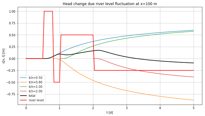
Fig. 6.19 Superposition in time example
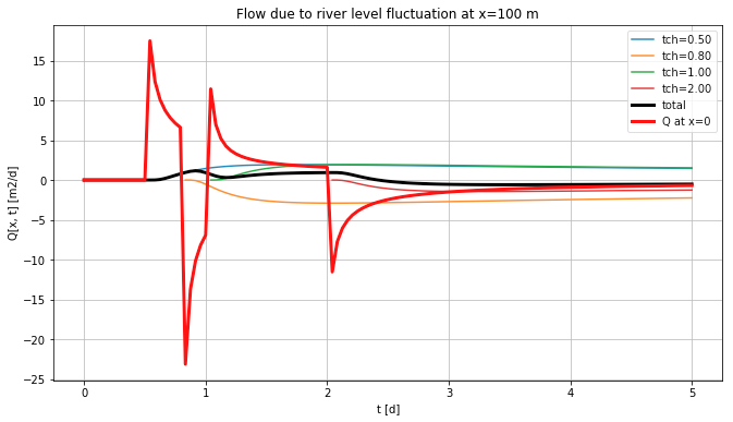
Fig. 6.20 Superposition in time example
6.5. Groundwater basins as land strips of limited width between straight head boundaries
6.5.1. Introduction
In many practical situations, groundwater basins will have a limited width instead of \(x\) extending to infinity. Examples are groundwater basins that are bounded by a fixed-head boundary on either side. This includes basins that are closed on one side, because such a line of no flow is just the water divide, which is equivalent to a symmetrical basin of double width having the same head boundary on either side.
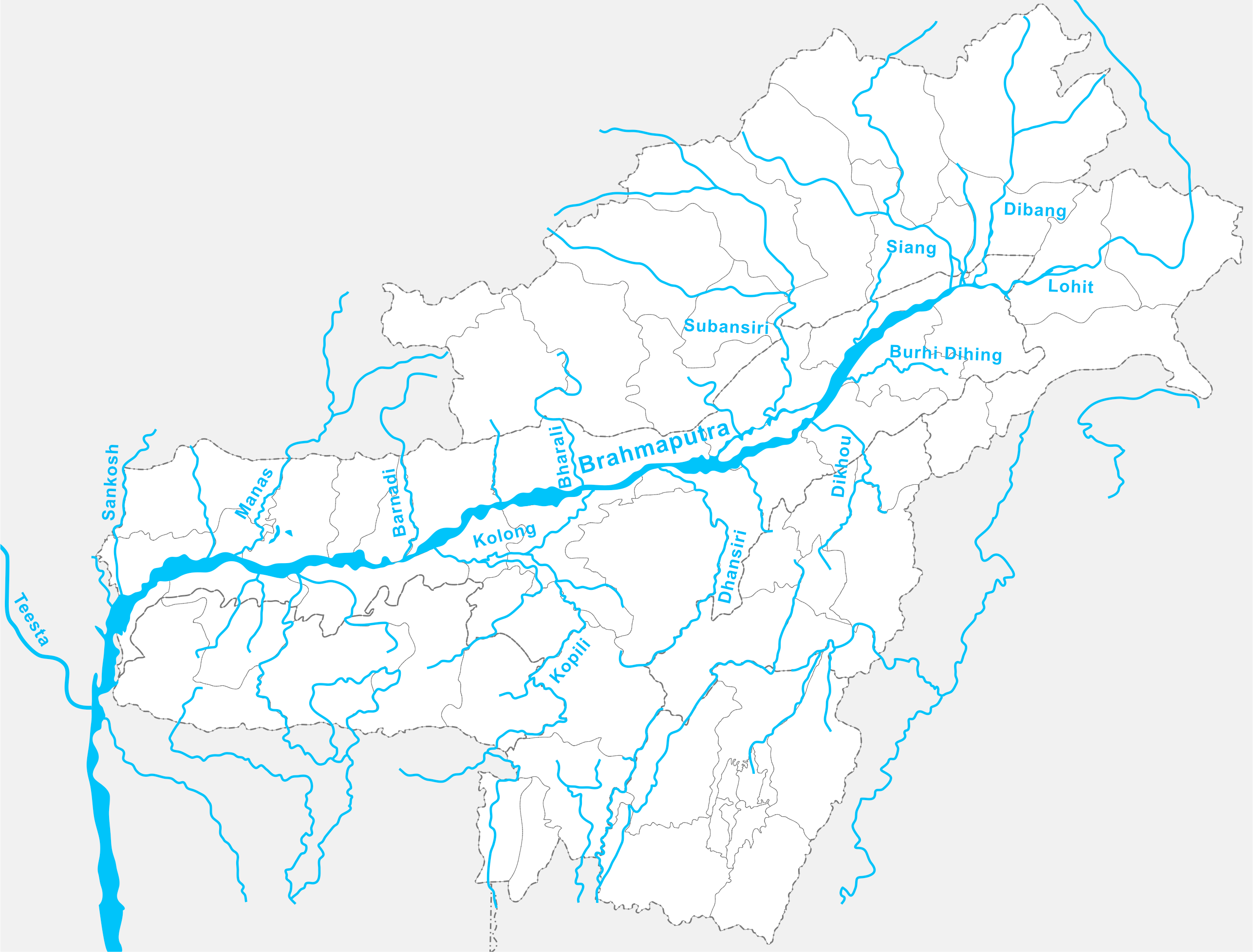
Fig. 6.21 Map of the Brahmaputra basin (Wikipedia)
Often, watersheds can be regarded as a set of sub-basins bounded by river branches on either side of the water divide between them (see Fig. 6.21). The basins considered here, can be regarded as a simplification of the groundwater system between two river branches, but also as a parcel of arable land bounded by two ditches. It’s just a matter of scale. The basins considered here may, therefore, be as narrow as a parcel of arable land or a meadow between ditches as one can find anywhere in the Netherlands of perhaps 100 m wide; but they can just as well be a strip of land land between brooks or tributaries that are several km apart, between river branches tens of km apart or a desert of which the boundaries lie at several hundred of km from each other.
Of course, the surface waters bounding most basins are not straight lines. Nevertheless, we limit ourselves to in this course to basins that are bounded by two parallel straight head boundaries. This makes the flow essentially one-dimensional when we ignore resistance due to vertical flow components with in the aquifer. The latter is very often justified because the vertical flow components are small compared to the horizontal ones. If this assumption is not valid like near a shallow surface-water body, where flow lines bend upward and convergence causing an extra loss of head, we may always add such effects separately.
In the following sections, we’ll learn how to compute the variation of head and flow in one-dimensional basins (basins in which the only spatial dimension is \(x\) and not \(y\) and \(z\), that are affected by the head changes at their two head boundaries, see Fig. 6.26) which shows such a basin (a strip of land) bounded on either side by a surface-water body in direct contact with the aquifer, such that the water level of these surface-water bodies determine the head at either side of the basin.
We first consider the case where the left-hand boundary head suddenly rises by a fixed amount \(A\) m, while the right-hand boundary head is kept the constant (see Fig. 6.22). We will see that maintaining the right-hand head boundary at zero, requires superposition of the effect of an infinite number of“mirror” strips of land. After that, we consider a given change of head on either side of the strip. This case is also solved by by superposition of an infinite number of equally sized land strips. The case in which the sudden head change is the same on either side of the land strip is just a special one. However, it allows us to compare it with a different general solution describing the drainage of a strip of land in which the head is initially uniform at a level \(A\) above its two boundaries. Both solutions are equivalent although they look mathematically completely different. The latter solution, however, allows drastic simplification when time is large enough and gives us a time constant that is characteristic of the basin, which allows analyzing time characteristics of any basin with a simple expression.
The mentioned superposition of an infinite number of strips leads to superposition patterns that are shown below the respective figure s. These patterns allow immediate recognition of the correctness of the superposition pattern required handle the head boundaries on both ends of the basin or the strip of land we want to analyze.
6.5.2. Water level at the left-hand side suddenly rises over a height of \(A\) m, while the water level at the right-hand side remains at zero
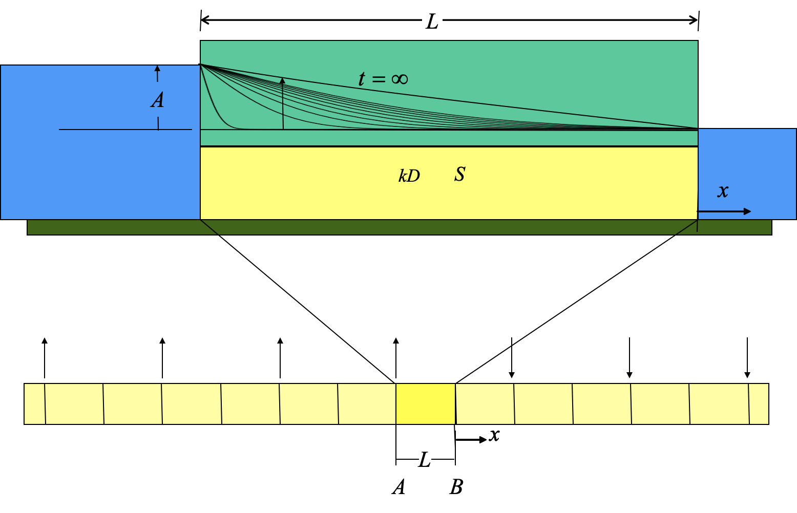
Fig. 6.22 Confined groundwater basin to the left and right bounded by surface water in direct contact with the aquifer. Here the water level at the left boundary is suddenly raised by \(A\) m at \(t=0\) and that at the right side the surface-water level remains unchanged at zero. The lower picture shows the superposition scheme in which the strip of length \(L\) between points A and B is the one to be analyzed. The arrows in the lower picture show where the water level is suddenly raised or lowered in the mirror scheme.
Fig. 6.22 shows a groundwater basin with a constant transmissivity \(kD\) and storage coefficient \(S\). It has a width \(L\) and is bounded on either side by surface water in direct contact with the confined aquifer. The water level at the left changes suddenly by an amount \(A\). How can we solve this, given the solution for the half-space (i.e. in which \(x\) runs from 0 to \(\infty\)) that we already have?
The answer is: by superposition by using mirror “ditches”.
The solution for the half-space has been shown before
However, this solution will cause the head at point \(B\) to start rising after some time, while in reality the head should remain 0 at point B. How wan we deal with this mathematically?
When we forget the surface water at \(x=B\), but instead assume a ditch at a distance \(L\) to the right of point B, in which the water level was suddenly lowered at \(t=0\) by an amount \(A\) m (i.e. changed by an amount - \(A\)), then the rising an point B due to the ditch at \(A\) would be exactly counterbalanced (neutralized) by the decline in point B due to the ditch at a distance \(L\) to the right of point B. As a consequence of both, the head at point B remains zero, which is exactly the desired effect. In this case, we have one mirror ditch with opposite head change at distance \(L\) to the right of point B.
However, this one mirror ditch does not solve the whole problem, because after some more time, it will cause the head at point A to start declining, and so the head at point A would not remain fixed at the value of \(A\) m.
To compensate for that, we need another mirror ditch at distance \(2L\) to the left of point A with opposite head change compared to to the first mirror ditch. But this head change at \(2L\) left of point A will cause the head at \(2L\) to the right of point B to change over time. This requires a mirror ditch at \(4L\) to the left of point A to neutralize this effect. And so on. We will, therefore, end up with an infinite number of mirror ditches just to make sure that boundary conditions at both sides of our initial basin are kept that their desired values.
The lower picture in Fig. 6.22 intends to make this clear. The darker yellow block represents the original basin of width \(L\). Each arrow represents a mirror ditch and its direction show whether the water level in it goes up or down.
Is this solution with the shown scheme of mirror ditches correct? Well, this is. In fact, it’s easy to see its correctness at a glance. Just look at the lower picture in Fig. 6.22 and consider point B, in which the head should remain zero. As it should become immediately clear by inspection, each ditch with lowered water level to the right of point B is exactly canceled at B by each ditch at the same distance to the left of point B with a rising level. Hence, the effect in point B of all ditches to the right is exactly canceled by all ditches to the left of point B. Therefore, the head at point B remains at zero.
On the other hand, all ditches to the right of point A are exactly compensated at point A by all ditches to the left of point A, except for the ditch at point A itself. Hence, the total effect of all the mirror ditches together at A is zero, so that the only remaining effect at A is that of the level rise at A itself. That too can be seen at a glance from the lower picture in Fig. 6.22.
With respect to the origin of the \(x\)-axis, it does not matter where we choose it, we need only to make sure that the distance \(x\) in the formula is correct for each of the mirror wells. In Fig. 6.22, the point with coordinate \(x=0\) was chosen at point \(B\), which makes the mirror ditches symmetrical with respect to this point. The \(x\)-coordinate of ditch \(i\) to the left is then
and that of ditch \(i\) to the right of point \(B\) is
The (absolute) distance to an arbitrary point with coordinate \(x\) is then for the left ditch
and to the right ditch
We can use these distances directly in the formula that sums the effect of all wells to yield the net result. This gives for the head change within the strip of land, where \(-L\le x\le0\):
and doing the same for the for the discharge expression, yields
Note that the second term in the formula for \(s\left(x,t\right)\) has a minus sign because of the water level in the right-hand ditches was lowered. However, the second term in the formula for the discharge \(Q\left(s,t\right)\) has a plus sign, because both the left-hand and the right-hand ditches cause a positive flow, i.e. a flow in the positive direction of the \(x\)-axis.
When you implement this scheme in Python, make sure you start the sum (loop) with \(i=1\) and not \(i=0\).
Fig. 6.23 shows the results for several times. Because the point \(x=0\) was chosen to be at the point B at the right-hand side of the strip, the \(x\)-values within the strip are now negative. Also notice that the steady-state solution, which is reached after about 3 days, has a head that declines linearly from 2.5 m at the left to 0 at the right of the strip. The discharge \(Q\) through the aquifer, therefore, must equal \(Q=A/L\times kD=2.5/250\times600=6\) m\(^{2}\)/d. This is indeed the case all along the width of the strip as can be seen in Fig. 6.23.

Fig. 6.23 Top: head. Bottom: flow. After sudden head rise of \(A=2.5\) m for various times, \(L=250\) m, \(kD=600\,\mathrm{m^{2}/d}\), \(Sy=0.1\)
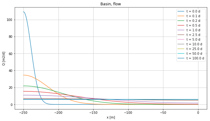
Fig. 6.24 Top: head. Bottom: flow. After sudden head rise of \(A=2.5\) m for various times, \(L=250\) m, \(kD=600\,\mathrm{m^{2}/d}\), \(Sy=0.1\)
6.5.2.1. Shifting the zero point of the \(x\)-axis
We may choose any point as the origin of the x-axis. Let’s put it at a distance \(a\) to the right of point A. The the coordinate of ditch \(i\) to the left would be \(x_{i}=-2iL-a\) for \(0\le i<\infty\) and that of ditch \(i\) to the right would be \(x_{i}=2iL-a\) for \(1\le i<\infty\). So that the distance between the first well a the right \(\left(i=1\right)\) and the first well at the left \(\left(i=0\right)\) equals
So with this zero point for the x-axis we can write the superposition as follows (note the start of the summation differs (1 at the left one and 0 at the right one)
removing needless minus signs in the distances
6.5.3. Arbitrary non-symmetrical case
Now consider the general case, in which the head at the left and right change by different values. Again, we need mirror ditches. This time not only to fix the left-hand head at the desired level, but also the right-hand head. Of course, you can regard this case from the perspective of the problem that we just solved. It is then the sum of the case in which the left-hand level was raised by \(A\) m and the right-hand level was kept at zero and the same case of which the right-hand size was raised by \(B\) m and the left-hand side was kept at zero.
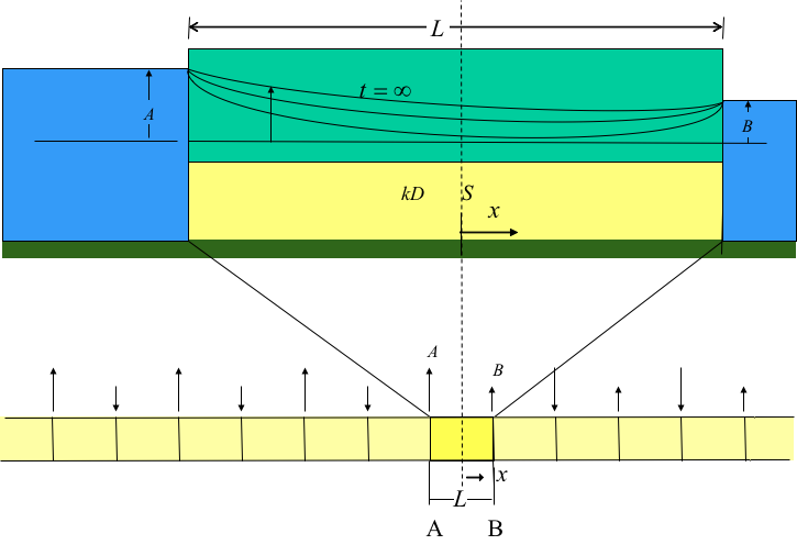
Fig. 6.25 As Fig. 6.22 but the water level is raised independently on the left and right side by \(A\) and \(B\) respectively, and the \(x\)-axis is now centered in the center of the strip. The lower picture shows the superposition scheme; the arrows show where the water level is suddenly raised or lowered.
But let’s just solve it, after taking the \(x=0\) at a convenient location, which would be in the center. Note however, you can put it at another location, but then the formulas change accordingly.
The image at the bottom of Fig. 6.25 shows the strip and the mirror ditches. By looking at this picture, it should immediately be clear that this scheme of mirror ditches is correct. To see this, look at point A. You will then notice that each ditch to the left of A is compensated exactly by each ditch at the right of A. Therefore, the only effect of all the ditches at point A, including the ditch at pint A itself, is that of the ditch at point A itself; all others cancel at point A. Next focus on point B and notice that this is also true for point B. Hence, at point A, the only effect that remains is that of the head change in the ditch at point A, and at point B, the only effect that remains at point B is that o the head change of the ditch at point B.
With this in mind, it becomes straightforward to write the expression for the head within the strip of land. To do that, just consider a point \(x\) and write the distance to all the ditches in terms of strip width \(L\) and \(x\). Doing this, we get
Like it was done above, a similar expression can be written down for the flow \(Q\).
An example result is shown in Fig. 6.26 for the case where at \(t=0\) the head at the left boundary was raised by \(A=2.5\) m and at the right side by \(B=1.5\) m. Again, a steady state is reached after about 5 days, the flow is then constant, i.e. \(\left(A-B\right)/L\times kD=1/250\times600=2.5\) m \(^{2}\)/d. The flows are initially, for a short period, high and opposite on both sides of the strip. Later on it became constant from left to right.
![[fig:Head-after-sudden-rise-left-and-right] Top: head Bottom: flow. After sudden head rise by :math:`A=2.5` m at :math:`x=-L/2` and :math:`B=1.5`\ m at :math:`x=+L/2` for various times, :math:`kD=600\,\mathrm{m^{2}/d}`, :math:`Sy=0.1`, :math:`L=250` m.](_images/StripSuperpositionLeftRight.png)
Fig. 6.26 [fig:Head-after-sudden-rise-left-and-right] Top: head Bottom: flow. After sudden head rise by \(A=2.5\) m at \(x=-L/2\) and \(B=1.5\)m at \(x=+L/2\) for various times, \(kD=600\,\mathrm{m^{2}/d}\), \(Sy=0.1\), \(L=250\) m.
![[fig:Head-after-sudden-rise-left-and-right] Top: head Bottom: flow. After sudden head rise by :math:`A=2.5` m at :math:`x=-L/2` and :math:`B=1.5`\ m at :math:`x=+L/2` for various times, :math:`kD=600\,\mathrm{m^{2}/d}`, :math:`Sy=0.1`, :math:`L=250` m.](_images/StripSuperpositionLeftRight_Q.png)
Fig. 6.27 [fig:Head-after-sudden-rise-left-and-right] Top: head Bottom: flow. After sudden head rise by \(A=2.5\) m at \(x=-L/2\) and \(B=1.5\)m at \(x=+L/2\) for various times, \(kD=600\,\mathrm{m^{2}/d}\), \(Sy=0.1\), \(L=250\) m.
6.5.4. Symmetrical case, \(A=B\)
The symmetrical case is obtained when the rise of the water level at the left-hand boundary is the same as that at the right-hand boundary, so \(A=B\). Of course, this case is included in the former one. However, we’ll still work it out as we need it in the next section to compare it with a completely different expression for the same case that we’ll use to generalize our understanding of the transient characteristics of groundwater basins.

Fig. 6.28 Groundwater basin bounded by surface water in direct contact on either side in which the water level is raised by \(A\) on both sides. The lower picture shows the superposition scheme with the errors indicating where the water level is raised or lowered for the superposition.
Fig. 6.28 shows the situation. It’s the same as before, but the rise is now \(A\) m on both sides, which simplifies the expression to a sum over two terms instead of four terms.
Taking \(x=0\) conveniently at the center of the strip like before, we can draw the mirror scheme. This is was done in the lower picture of Fig. 6.28. Like before, by first focusing on the symmetry around point A and then on the symmetry around point B, you should see at a glance that this mirror scheme is correct. Knowing the mirror scheme, we can write the expression (See also Carslaw and Jaeger, p97, eq 9):
The factor \(\left(-1\right)^{i-1}\) is just a series \(+1,-1,+1,-1,+1,-1,\dots\) because the direction of the arrow alternates with each further ditch on both sides.
6.5.4.1. Another perspective, drainage of a basin in which the head is initially at distance A above the fixed heads at either side of the strip
This case, in which the water level at both boundaries suddenly rises by the same amount of \(A\) m, can also be regarded as a transient drainage after a heavy shower of rain on the strip. If we assume that the rain surplus \(P\) [m] reaches the water table immediately, then the water level in the entire strip would suddenly rise by the amount \(A=\frac{P}{S_{y}}\) in which \(P\) is the rain (that part of it that reaches the water table) and \(S_{y}\) is the specific yield. Therefore, after such a shower, the head in the entire strip would suddenly be at \(A\) m above the water level in the ditches on either side. Immediately after this shower, assumed to be of zero duration, the strip starts draining. The picture that is thus obtained is the same as that in which the ditches suddenly rise by \(A\) m at \(t=0\), be it that the drainage picture is turned upside-down. This drainage situation is illustrated in Fig. 6.29.
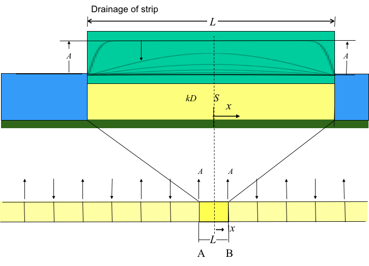
Fig. 6.29 Symmetrical strip draining after heavy shower.
To use this equation to compute the drainage of a groundwater basins one may write \(s\left(x,t\right)=A\left(1-\sum\dots\right)\), where \(\sum\dots\) is the entire expression in the formula above.
The discharge at any point \(x\) is obtained as usual by inserting using Darcy’s law, i.e. \(Q=-kD\left(\partial s/\partial x\right)\):
As can be seen from Fig. 6.26, immediately after the head change, the water table drops very fast near the edges of the strip. Very soon, however, the head takes the shape of a cosine and the strip drains gradually until its final equilibrium at \(s\left(x,t\rightarrow\infty\right)=0\) is reached.
The cosine shape at later drainage stages follows from another form of analytical solution of the same strip, which will be discussed in the next section.
An example is shown in Fig. 6.30. In this case, the time interval between times used to show the heads is the so-called halftime as will be derived later. After each halftime, the difference between the head and the equilibrium final head is halved.
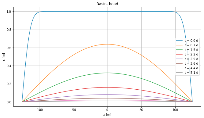
Fig. 6.30 Top: head. Bottom: flow. Drainage after a sudden shower of 100 mm, such that with \(S=0.1\), \(A=1\) m at \(t=0+\). Thereafter, the strip drains towards the surface water at both sides, the water level of which is kept constant. \(kD=600\,\mathrm{m^{2}/d}\), \(S=0.1\), \(L=250\) m. Situation for several times.
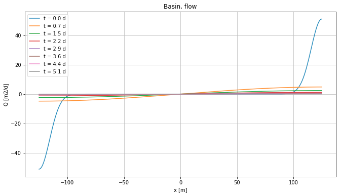
Fig. 6.31 Top: head. Bottom: flow. Drainage after a sudden shower of 100 mm, such that with \(S=0.1\), \(A=1\) m at \(t=0+\). Thereafter, the strip drains towards the surface water at both sides, the water level of which is kept constant. \(kD=600\,\mathrm{m^{2}/d}\), \(S=0.1\), \(L=250\) m. Situation for several times.
6.5.5. Questions
Set up a mirror scheme for the case of a strip of land bounded by straight surface water on either side, where the surface water stage of the right-hand side canal suddenly changes by a fixed value.
Show, explain on the hand of the obtained mirror scheme that the result is correct, i.e. that the result with all the mirror strips match the boundary conditions exactly.
What would be the mirror scheme for the strip if the right-hand boundary was closed?
6.6. Symmetrical drainage from a land strip bounded by straight head boundaries (characteristic time of flow basins)
Here we introduce a solution for the drainage of a land strip that initially has uniform head \(s\left(0,x\right)=A\) and is bounded by two straight head boundaries at \(x=\pm b\) with head at \(s\left(\pm b,t\right)=0\). This solution looks completely different from the one we obtained by infinite mirroring of strips of land as we did in the previous sections, yet it provides the same result for the symmetrical case. The advantage of this form of the solution is that it can be further analyzed to deduce general drainage patterns and their time scale.
6.6.1. Analytical solution
An analytical solution for the drainage of a strip of land that we solved by superimposing an infinite number of mirror ditches is also known in a completely different mathematical form published by Carslaw and Jaeger (1986), p97, eq. 8. It was also published by Verruijt (1999), p87 and is widely known in the Netherlands as“Kraaijenhoff van der Leur”. It reads
From this we obtain the flow by setting \(Q=-kD\frac{\partial s}{\partial x}\). This yields
As always, \(s\left(x,t\right)\) is the head relative its equilibrium value, which is \(s\left(x,\infty\right)=0\). The \(x\)-axis is taken such that \(x=0\) in the center and \(x\pm b\) corresponds to the sides with fixed boundary conditions \(s\left(\pm b,t\right)=0\). The initial head is \(s\left(x,0\right)=A\) inside the section, \(-b<x<b\). The formula describes the drainage that follows after the initial situation.
This behavior is characteristic for a basin after a sudden shower causing the head in it to suddenly rise everywhere by the same amount, while the level in the ditches at both sides is kept the same. After the shower, the drainage sets in and gradually continues until equilibrium is finally reached (which theoretically takes infinite time).
(6.13) yields the same head as was obtained previously with superposition of an infinite number of erfc-functions, even though the solution presented here looks mathematically completely different. We will use this solution to derive drainage characteristics that can be applied in practice on different scales.
Fig. 6.32 gives the results as an example. The lines are the same as in Fig. 6.30 and the dots are the results of (6.13) for the same times. The results are, obviously, the same. The lower picture in this figure shows the computed discharge using both approaches.

Fig. 6.32 Top: head. Bottom: flow. Free drainage of basin from initial head at \(A=1\) m for various times, \(kD=600\,\mathrm{m^{2}/d}\), \(Sy=0.1\), \(L=250\) m. Drawn lines were computed with the \(\mbox{erfc}\)-functions and are the same as in Fig. 6.29; the dots were computed with (6.13). The lines from both approaches completely overlap.
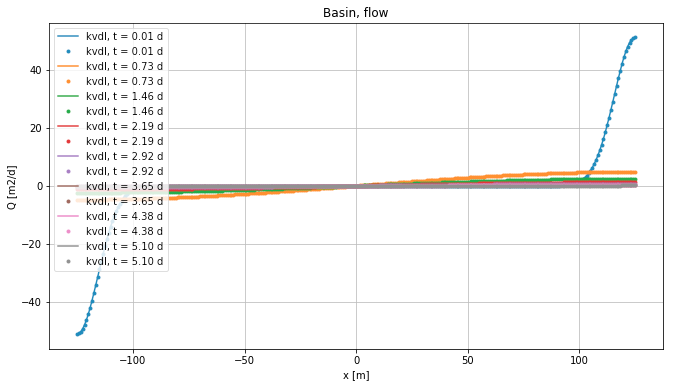
Fig. 6.33 Top: head. Bottom: flow. Free drainage of basin from initial head at \(A=1\) m for various times, \(kD=600\,\mathrm{m^{2}/d}\), \(Sy=0.1\), \(L=250\) m. Drawn lines were computed with the \(\mbox{erfc}\)-functions and are the same as in Fig. 6.29; the dots were computed with (6.13). The lines from both approaches completely overlap.
Finally, Fig. 6.34 shows a graph of the individual terms of the series in (6.13) for head and for discharge \(Q\), both together with the total solution obtained by the summation a large number of terms.
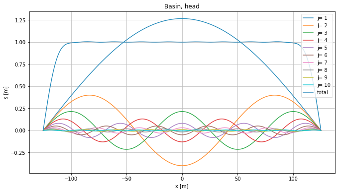
Fig. 6.34 Showing the individual terms of the series in (6.13) for head and for flow together with the total solution obtained by the summation. This is done for \(t=0.0073\) d. Other values are the same as in Fig. 6.32.
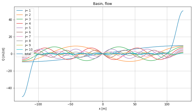
Fig. 6.35 Showing the individual terms of the series in (6.13) for head and for flow together with the total solution obtained by the summation. This is done for \(t=0.0073\) d. Other values are the same as in Fig. 6.32.
6.6.1.1. Exercise:
Implement (6.13) yourself together with the solution using superposition of mirror ditches and show that the outcomes are the same when simulation free drainage of a strip of land. You should obtain Fig. 6.32.
6.6.2. Long-term drainage behavior, characteristic drainage time
(6.13) looks complicated at first, but it can be broken down to yield useful and practical insights pertaining to the dynamic characteristics of draining groundwater basins. For that purpose, we analyze the expression under the summation.
The \(2j-1\) is just the series \(1,3,5,7,\dots\). and \(\left(-1\right)^{2j-1}=+1,-1,+1,-1,\dots\). Next, we have a product of a cosine and an exponent. The cosine will fluctuate between -1 and +1 and it only depends on \(x\). Then notice the exponent, which only depends on time. For simplicity write it as
where \(T=\frac{b^{2}S}{kD}\). \(T\) may thus be regarded as a characteristic time of the drainage. The exponent terms in the series now become
Because \(\frac{t}{T}>0\), the second and higher terms will finally become much smaller than the first and may, therefore, be neglected when \(t>t_{n}=nT\) where \(n\) needs to be estimated. So let us see when the second term becomes much less than the first one, so that only the first term matters and we can neglect all higher terms. Therefore, compare the first term with the second and demand that it’s much larger than the second:
or
where \(G\) is just a large positive number. We may choose \(G=100\), which means, we neglect all higher terms, when the first term is at least 100 times a large as the second.
Taking the logarithm at both sides of the equal-sign yields
Hence, we obtain
so that
This way, for the chosen value of \(G=100\), we find \(t=0.23T\). Therefore, we conclude that all higher terms are negligible when \(t>0.23\,T\). Of course, we could also have chosen another large value of \(G\), but the outcome would not be much different because \(G\) is under the logarithm.
This means that when \(t>0.23T\) the expression given above reduces to only one term
This is a simple-to-understand expression. It is a cosine that only depends on \(x\), not on time, with its top equal to \(\frac{4}{\pi}A\) in the center where \(x=0\) and zero where \(x=\pm b\). This cosine-shaped groundwater mound gradually declines according to the exponent that only depends on time, not in \(x\).
An exponential decline can always be characterized by its so-called halftime. The halftime is the time in which the head reduces by a factor 0.5. So if \(t\) increases by one halftime, \(\Delta t_{50\%}\), the head \(s(x,t)\) is reduced to \(0.5\times s\left(x,t\right)\).
To obtain this halftime, just write down mathematically that half the head at time \(t\) is obtained at time \(t+\Delta t_{50\%}\). So literally
Taking the logarithm on both sides yields
and so
and, therefore,
or
This implies that when time progresses by \(\Delta t_{50\%}=0.28T\), the drawdown is halved (under the condition that \(t>0.23T\) when all higher terms can be neglected).
This result allows us to immediately compare the halftimes of the free drainage of groundwater basins of widely different sizes and with widely different aquifer properties. Let the size of the basin be expressed by its representative half-width \(b\). Of course, when a groundwater basin does not have has the shape of a long strip bounded by two straight canals, one should estimate a reasonable half-width based on the distance from the water divide to its drainage base, be it ditches, canals, streams, lakes, rivers or the coast.
Table 6.1 gives the characteristic time \(T=b^{2}S/kD\) and the halftime \(\Delta t_{50\%}=0.28T\) for some groundwater basins. This table illustrates, that different groundwater basins that may have similar transmissivities and storage coefficients, may still have extremely large differences in half times or characteristic times. Especially the effect of the width of the basins, \(b\), is large because it works to the power 2 in \(T=b^{2}S/kD\). This way, a simple meadow or arable field in the Netherlands bounded between two ditches just 100 m apart may have a halftime in the order of one day, but large systems, notably deserts, like the Kalahari may have a halftime in the order o 10000 years. This implies that the small meadow in the Netherlands, will hardly remember the rain shower that fell one week ago, while the Kalahari is still draining the water that it collected during previous wet episodes may thousands of years ago, like the last ice age. Recent research with respect to the world’s largest aquifer, the Nubian sandstone, showed that this aquifer, which extends over much of Sudan, Egypt and Libya, may be regarded as a water-table aquifer that is still slowly draining the water that it collected during wet episodes when the Sahara was still wet (especially between the beginning of the Holocene era until about 4600 years ago, (Powell and Fensham 2015; Voss and Soiman 2014) and that the current oases represent the last remains of the water table reaching above ground surface, and which was much higher thousands of years ago.
Situation |
Country |
\(kD\mathrm{[m^{2}/d]}\) |
\(Sy\) |
\(b\mathrm{[m]}\) |
\(T\mathrm{[d]}\) |
\(T_{50\%}%\mathrm{[d]}\) |
\(T\mathrm{[yr]}\) |
\(T_{50\%}%\mathrm{[yr]}\) |
|---|---|---|---|---|---|---|---|---|
Nubian Sandstone |
Egypt |
500 |
0.001 |
500,000 |
500,000 |
140,000 |
3845 |
420 |
Kalahari Desert |
Botswana |
500 |
0.1 |
300,000 |
\(18\times10^{6}\) |
540,000 |
14000 |
15000 |
Veluwe Area |
NL |
6,000 |
0.27 |
20,000 |
18,000 |
5,040 |
14 |
15 |
Dunes (NL coast) |
NL |
200 |
0.11 |
2,000 |
4,400 |
1,200 |
3 |
4 |
Flower bulb fields |
NL |
200 |
0.1 |
50 |
1.25 |
0.35 |
0.001 |
0.001 |
6.6.3. Questions
Show on the hand of (6.13) what the half-time of the drainage of this system is. Derive it yourself.
How does the characteristic time relate to halftime? Show this mathematically?
Implement (6.13) and make a graph of some of the first terms of the series and of its sum.
Show that (6.13) equals (6.11) by implementing both, which you may do using a language like Python or a spreadsheet like Excel. Notice that the \(\mbox{first}=1-\mbox{second}\).
Derive the discharge from (6.13) and show that it is the same as that in (6.12) by implementing both in the same spreadsheet.
Show some of the first terms of the series in (6.11) in Python or Excel.
7. Transient flow to wells
7.1. Introduction
This chapter deals with the flow to wells in aquifers. The flow to a well is treated as axially symmetric and horizontal. Vertical resistance to flow within the aquifer itself is neglected in this course. This is the so-called Dupuit-Forchheimer approximation. It is a very useful approximation because it allows computing regional groundwater flow in aquifers accurately in a vertically integrated manner by considering the flow to be horizontal (or more exactly: by neglecting the resistance to vertical flow). This way, we don’t have to deal with head losses due to vertical flow components. Important vertical components may, however, occur in the vicinity of wells that only partially penetrate the aquifer. Disturbances of the essentially horizontal flow due to partial penetration of well screens is, however, only important in the vicinity of the wells, at distances less that 1.5 times the aquifer thickness, and can be dealt with by a correction on the drawdown as will be outlined in the facultative Partial penetration of well screens (section ) .
We will handle more complicated situations, such as well fields and wells near specific boundaries, by superposition of mirror wells. By the way, also partial penetration is effectively handled by superposition.
We start this chapter with an overview of the analytical solutions that we will deal with and their related steady-state versions.
In the past, the actual computation of groundwater-flow solutions by looking up the values if the functions in tables. Nowadays, because everyone has access to powerful computational software like Excel or Python, we will compute the values of the different well functions using those it, rather than looking them up in tables. However, tables remain extremely important as a means to verify our own numerical implementation of solutions and functions. Further, not all required mathematical functions may be available in our actual computational program, especially not in Excel. In that case we can implement those functions ourselves. This may be done in Excel using Visual Basic. However, in the exercises of this course we’ll use the much more powerful Python language inside digital notebooks. Notice that Python is freely available and can be downloaded from the Internet. Generally, only a few lines if Python code are needed to implement and use the most important transient groundwater-flow solutions and apply superposition in time and or in space to handle more demanding situations.
7.2. Wells and well functions overview

Fig. 7.1 Large-diameter open well in India (copied from newspaper NRC some years ago).
The next three figure s provide an impression of what wells are, without entering into the details of their construction or the installation of pumps, pump cellars, electricity and so on. What matters for us, is the position of the screen inside the aquifer. There exist numerous types of wells: open wells, dug wells, drilled wells, tube wells, horizontal wells and more. In this course, we limit ourselves to wells of small radius, in which water storage inside the well-bore can be neglected. This limitation suffices for most practical situations. Many more solutions for special cases can be found in Carslaw and Jaeger (1986) and in Bruggeman (1999). With respect to well testing and pumping-test analyses there is the world-famous book Kruseman and Ridder (1970). It has been used in all continents since 1970. The second edition of this book (Kruseman and Ridder 1994), can be downloaded from the Internet for free (https://www.hydrology.nl/images/docs/dutch/key/Kruseman_and_De_Ridder_2000.pdf). The book is a very good reference, which covers the relevant literature on pumping-test analyses. Furthermore, it is practical and provides tables with the values for many of the analytical groundwater functions that you may ever need to check your own implementations.
The analytical solution for large-diameter wells, is such a special case, which is useful for situations like the one illustrated in figure . The implementation of the solution for large-diameter wells with in-bore water storage is provided in Large-diameter wells (not for the exam), just for reference, not as part of this course.
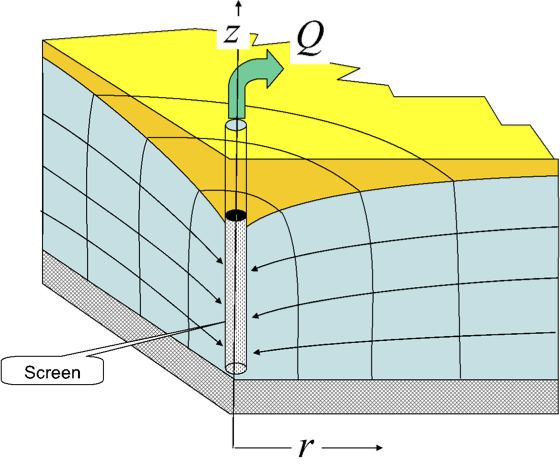
Fig. 7.2 A tube well in an unconfined aquifer
Fig. 7.2 is a sketch of a (tube) well in an unconfined aquifer (“unconfined” is synonymous with“water-table aquifer” and with“phreatic aquifer”). A“confined aquifer” does not have a water table, its top is given by the bottom of an overlying layer. A semi-confined aquifer is also confined, but the layer on top is leaky, as may be this also holds for the layer at its bottom.
Fig. 7.3 gives a sketch of a tube well in a (semi)-confined aquifer. The difference between a confined and a semi-confined aquifer, is that the top and bottom of the confined aquifer are both impervious (there is no vertical leakage), while the semi-confined aquifer has vertical leakage through its ceiling, its floor or both. The screen, i.e. the perforated portion of the well is considered to be fully penetrating the (wet) thickness of the aquifer, see Fig. 7.2. The well’s screen is not completely penetrating the aquifer in Fig. 7.3. This is very often the case in practice, where well screens only partially penetrate the aquifer because this saves drilling, material and installation costs where the aquifers are much thicker than is necessary for the designed extraction rates. It should be noted however, that due to partial penetration of a well screen, the streamlines in the vicinity of the screen will no longer be all horizontal. The concentration of the streamlines towards the top and the bottom of a partially penetrating well screen causes extra head loss relative to the situation with a fully penetrating well screen. This head loss can be taken into account when necessary as outlined in the facultative Partial penetration of well screens .

Fig. 7.3 Tube well with stream lines in a semi-confined and a confined aquifer
The right-hand side of Fig. 7.3 shows the streamlines in the case of a completely confined aquifer, one without vertical leakage. The left-hand side of Fig. 7.3 shows the streamlines in a semi-confined aquifer that is recharged by seepage from an overlying layer. Of course, seepage may also occur from underlying layers. In practice we may encounter multi-aquifer systems, in which aquifers are sandwiched between semi-pervious layers. However, we will not deal with such multilayer groundwater-flow systems in this syllabus. The modern theory for multilayer aquifer systems may be looked up in (Hemker 1984, 1985; Hemker and Maas 1987) in (Hemker and Maas 1987) and in Bruggeman (1999).
It is important to realize that flow due to an extraction by a well in a water-table aquifer or a perfectly confined aquifer of infinite lateral extent will never reach equilibrium; it will always remain transient. The reason is that all the water has to come from storage. Or more precisely, the extraction by itself does not cause any water external to the aquifer to enter the aquifer. Even rain does not have any effect on the drawdown caused by the extraction. Of course, rain does change the head in the aquifer, but this change is completely independent of the extraction from the well. This recharge has an effect that can be superimposed independently from the that caused by the extraction. Only when a well extraction causes water to flow across aquifer boundaries as an effect of the gradients created by the well extraction, can the flow reach an equilibrium, i.e. steady state after a limited time. Therefore, a continuous extraction from a confined aquifer of infinite extent never reaches steady state, but a continuous extraction from a semi-confined aquifer does reach steady state, as does an extraction by a well in an aquifer that is bounded by some fixed-head boundaries. Of course, if the flow through the semi-confined layer drains higher-up layers or even an overlying marsh, then this steady-state situation may not be reached, or it cannot be maintained for a very long time as the overlaying swamp itself would be drained by the leakage created by the well extraction in from the aquifer below. In that case, we will see a delayed yield, which is outlined in the facultative Delayed yield (delayed water-table response)on . In practice, it is always important to realize that extraction from a semi-confined layer may drain overlying layers such that the head in or above the overlying layer will also decline, which in turn will cause the induced leakage through the confining layer to decline and even stop entirely over time. The more the leakage declines due to the delayed drainage of overlying layers, the more the head in the aquifer will start behaving like a confined or unconfined layer without vertical leakage but with the specific yield of the overlying layer as its storage coefficient, hence the expression“delayed yield”.
Governing partial differential equations are important as they express the physical foundation and the approximations made to solve a problem analytically as well as numerically. They will be presented further down. However, the general relation between solutions for a water-table aquifer and a confined aquifer is presented first.
7.3. General relation between the well-induced head change in a water-table and confined aquifer and the relation between the different analytical solutions for drawdown by a fully penetrating pumping well
The transmissivity in a water-table aquifer is given by \(T=kh\) where \(h\) is the distance from the water table to the bottom of the aquifer; while in the derivation of solutions the bottom of the aquifer is assumed to be horizontal. The transmissivity of a confined aquifer is \(T=kD\) with \(D\) its thickness and the transmissivity, which is assumed constant. In an unconfined aquifer, the thickness and head \(h\) depends on distance between the water table and the bottom of the aquifer. In a water-table aquifer, the thickness does in fact vary with the water table as it changes due to the pumping, and perhaps also due to other factors like varying boundary conditions.
It should be noted that there exist no analytical solutions dealing with a time-variable water table; all available solutions approximate the water-table situation by taking \(D\approx h\), where \(h\) should be a suitable average over the area of interest.
To allow an analytical solution for a transient groundwater problem to be found, the governing partial differential equation is linearized before solving it. Superposition can then be applied using the solutions of the linearized partial differential equation.
Superposition allows us to add up an arbitrary number of different solutions to the same groundwater system in order to handle more complex situations. When the underlying governing partial differential equation is linear, the effect of individual wells remain completely separated from effects of other factors or boundary conditions. This implies that precipitation and evaporation play no role when it comes to computing the changes of the groundwater heads and flows caused by wells.
This simplification may fail when the groundwater system does not obey the assumptions that underlie our partial differential equation. This is the case, for example, when plant evaporation is reduced in a nonlinear fashion by the drawdown of the water table. One should keep such exceptions in mind when solving practical problems and stay aware of the limitations to the calculation methods and formulas applied. Of course, the same is true when applying groundwater models.
Table 7.1 shows the most important groundwater-well solutions. Only the first one in the table deals with a water-table aquifer; all other well solutions require the transmissivity to be constant. To use these solutions for water-table aquifers, the drawdown must remain small compared to the wet aquifer thickness; it may not change by more than say 20% of the original aquifer thickness. However, one may often overcome such conditions by using a proper average for the aquifer thickness. The water-table solution in the table depends on \(h^{2}-H^{2}\). Note that this can be converted into a product of the drawdown and the aquifer thickness as follows
By replacing \(h^{2}-H^{2}\) in the first solution by \(2sH\) one obtains the second. (7.1) also gives a clue with respect to the accuracy of using a confined-aquifer solution for the water-table case, which we will often do in practice. It requires that \(h+H\approx2D\). A head change of \(h\) of 20% of \(H\) therefore, causes an error in the computed drawdown of about \(10\%\), which is acceptable under most circumstances.
Clearly, the second Thiem solution in the table below is directly related to the transient Theis solution, but they are not equivalent, because the Theis solution has no steady state. However, the difference between the transient heads at two finite distances from the pumping well does become steady state over time, and that steady state is equivalent to the Thiem solution for constant aquifer thickness. The steady-state solution for the flow to a well in a leaky aquifer, according to De Glee (1930) in the table, is the steady-state equivalent of the transient solution of Hantush (1955). Also notice that all steady-state solutions have a 2 in the denominator of the factor multiplying the well function or the logarithm, while all transient solutions have a 4 at that position. From this, it immediately follows that the Hantush solution for \(t\rightarrow\infty\) is
so that
where \(\mbox{W}_{h}\left(r,\frac{r}{\lambda}\right)\) is the Hantush well function and \(\mbox{K}_{0}\left(\frac{r}{\lambda}\right)\) is the modified Bessel function of the second kind and zero order.
Name |
Water-table? |
Leakage? |
Transient? |
Solutions |
|---|---|---|---|---|
Thiem |
yes |
no |
no |
\(h^{2}-H^{2}=\frac{Q}{\pi k}\ln\frac{R}{r}\) |
Thiem |
no |
no |
no |
\(s=\frac{Q}{2\pi kD}\ln\frac{R}{r}\) |
De Glee (1930) |
no |
yes |
no |
\(s=\frac{Q}{2\pi kD}\mbox{K}_{0}\left(\frac{r}{\lambda}\right)\) |
Theis (1935) |
no |
no |
yes |
\(s=\frac{Q}{4\pi kD}\mbox{W}\left(u\right)\) |
Hantush (1955) |
no |
yes |
no |
\(s=\frac{Q}{4\pi kD}\mbox{W}_{h}\left(u,\frac{r}{\lambda}\right)\) |
7.4. Theis and Hantush wells in an infinite aquifer with constant transmissivity and storativity; the governing partial differential equation
7.4.1. Introduction
In 1935, Theis (1935) published a new solution for the dynamic change of head \(s\) [m] caused by a well that, at \(t=0\), begins pumping at a constant rate \(Q\,\mathrm{[L^{3}/T]}\) from an infinite aquifer having uniform transmissivity \(kD\,\mathrm{[L^{2}/T]}\) and storativity \(S\,\mathrm{[-]}\).
The solution by Theis has been a major breakthrough in groundwater hydrology. For the first time, it became possible to analyze the dynamics of the heads and flows caused by extracting wells. Before Theis, only steady-state flow solutions for the groundwater flow to wells existed, which very much limited possible analyses of actual pumping regimes. According to Theis, when a well pumps from an aquifer of infinite extent, all water must come from storage; there are no extra sources of the extracted water.
Then, 20 years layer Hantush (1955) developed an analytical solution for the flow to a well in a semi-confined aquifer. The only difference between the two being that with Hantush, the water would not only come from storage from the aquifer itself, but also from leakage through an overlying (and or an underlying) aquitard in proportion to the drawdown caused by the well. This solution also largely extended the possible cases that were amenable to analyses. Contrary to the Theis-solution, the Hantush solution does approach a steady state within a limited time. Both solutions are mathematically similar, in fact, the Theis solution is a special case of the more general Hantush solution; the Theis solution is the Hantush solution for the case that the vertical hydraulic resistance of the aquitard \(c=\frac{d}{k'}\) [T] (with \(d\,\mathrm{[L]}\) the thickness of the aquitard and \(k'\,\mathrm{[L/T]}\) its effective vertical conductivity) is infinite. Note that the dimension of \(c\) is [T], i.e. time. The flow and drawdown caused by extracting from a well in an infinite aquifer must be axially symmetric. Fig. 7.4 shows the general situation in cross section. A well with a well radius \(r_{0}\) is extracting a constant flow \(Q_{0}\,\mathrm{[L^{3}/T]}\). The aquifer is semi-confined; so there is exchange of water through the overlying aquitard with resistance \(c\) [T] with water on top of that layer with a constant water level \(h_{0}\). All water levels or heads are with respect to an arbitrary datum (reference elevation) as indicated. The leakage at any \(t\) and \(r\) equals \(n=\frac{h_{0}-h_{r,t}}{c}\) [L/T]. The head in the aquifer is denoted by the curved lines. During the time step \(dt\) the head increases from \(h_{r,t}\) to \(h_{r,t+dt}=h_{r,t}+\frac{\partial h_{r,t}}{dt}dt\). Please watch the signs. It is clear that when we extract water from the well, the heads will decline and the flows designated in the figure are directed towards the well. However, they are drawn in the opposite direction, the direction in which \(r\) is positive and \(h\) is positive. This facilitates somewhat the derivation, it only has an effect on where we will have minus signs.
7.4.2. The governing partial differential equation
We start the derivation using small discrete values for the distance difference \(\Delta r\) and the time step \(\Delta t\), which later on will be reduced to the infinitesimal values \(dr\) and \(dt\) respectively. Furthermore let \(Q\) be the flow in the middle of our time step.
Now consider the water budget for a ring between \(r\) and \(r+\Delta r\) surrounding the well expressed in rates. The water budget in terms of rates for the ring then is as follows (using \(h\) for the head):
\(\mbox{rate of inflow from the right}\) + \(\mbox{ rate of inflow from the left}\) = \(\mbox{ rate of leakage to adjacent layer}\) + \(\mbox{ rate of storage}\)
dividing by \(2\pi r\Delta r\) and by \(kD\) yields
Taking the limit for \(\Delta r\rightarrow dr\) yields the partial differential equation
We may set \(s=h-h_{0},\) showing that the solution depends on the difference between the head in the aquifer and that in the adjacent layer. Therefore, our final partial differential equation is in terms of the head difference with the constant head in the adjacent layer becomes
This partial differential equation is valid for axial flow in a semi-confined aquifer, and therefore, also for the Hantush (leaky) situation. It should be immediately clear that for \(c\rightarrow\infty\), i.e. when the aquitard becomes impervious, turns into an aquiclude, the term \(s/\lambda^{2}\) drops out. This then yields the partial differential equation that is valid for the Theis situation. Hence, the Theis situation is a special case of the Hantush situation.
It should further be clear from this derivation that the partial differential equation is a water budget on infinitesimal scale. The left-hand side tells us how much the net flow of water is that flows into one meter of the the ring (not out of the ring, because in the last but one equation above we changed the sign), while on the right-hand side of the equal sign we have the terms that quantify where this net inflow goes. The first term to the right gives the part that flows into storage, and the second term to the right quantifies the leakage lost to the adjacent layer. With the second term on the right-hand side zero in the case of the Theis situation, all net water flow into the ring goes into storage and, vice versa, all water extracted from the ring (i.e. from the aquifer) stems from storage and only from storage.
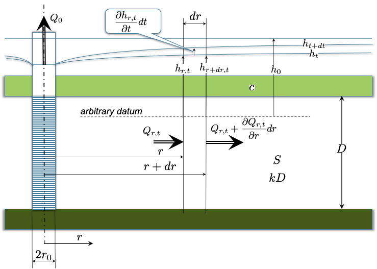
Fig. 7.4 Transient axial flow to a fully penetrating well in a semi-confined aquifer.
In the derivation derived above, we considered a (semi-)confined aquifer, i.e. an aquifer filled to the top without a free water table. The storage coefficient, therefore is the elastic storage coefficient \(S\) [-], i.e. the specific storage coefficient \(S_{s}\) [1/L] multiplied by the aquifer thickness \(D\) [L]. If we substitute the specific yield \(S_{y}\) [-], which is also dimensionless, for \(S\) [-] the partial differential equation is just as valid for a water table aquifer, under the sole condition that the thickness of the water-table aquifer may be regarded constant, just like the transmissivity in the case of a confined or semi-confined aquifer. Generally, for this assumption to be acceptable, the drawdown due to the well extraction must not be too large with respect to the thickness of the aquifer. A drawdown below 20% of the wetted thickness of a water-table aquifer usually is acceptable, especially when we apply the linearization explained in the previous section.
7.4.3. The Theis and Hantush well functions
Now with the governing partial differential equation in place, the art is to find closed analytical solutions for specific cases that are useful to us, for instance the flow towards wells. These solutions then must fulfill both the partial differential equation and the initial conditions and the boundary conditions. A useful solution of a well would be that for which the initial head or drawdown is zero, and as boundary conditions that the head at infinity will always remain zero, while the flow through a ring with infinitesimally small radius around the well equals the constant extraction from the well. This solution was found by Theis (1935) for the Theis situation (i.e. without leakage) and by Hantush (1955) for the Hantush situation (i.e. with leakage through an aquitard from an adjacent layer with constant head).
The Theis solution is generally written as
in which \(\mbox{W}\left(-\right)\) is called Theis’ well function among hydrogeologists, see below. Note the small \(s\) [L] stands for change of head, while the big capital \(S\) [-] is used for the storage coefficient of the aquifer.
As just said, the function \(\mbox{W}\left(\right)\) is known as Theis’ well function among hydrologists. However, mathematicians new that function long before Theis; they have a name for it, namely the exponential integral, it can be expressed as an integral
This well function is given in tables in books that describe pumping test analyses like Kruseman and Ridder (1994) as well as in books with mathematical tables like the famous Abramowitz and Stegun (1972). Nowadays, this exponential integral function is readily available in software such as Python, but in Excel it has to be implemented by yourself, which may be done in Visual Basic.
The Hantush solution function is similar, it can be expressed as
in which \(\mbox{W}_{h}\left(\right)\) is called the Hantush well function, which now depends on both \(u\) and \(\lambda\). Mathematically, the Hantush well function is similar to to the Theis well function, it is written as
It is immediately clear, that when \(c\rightarrow\infty\), so that \(\lambda\rightarrow\infty\), we get the Theis well function back. Hence, Theis is a special case of Hantush.
The conditions under which the drawdown formulas are valid are summarized as follows:
The aquifer has uniform transmissivity and uniform storativity (either elastic storativity (or storage coefficient) when confined/semi-confined, or specific yield when phreatic). In case of a phreatic/unconfined/water-table aquifer, the drawdown should be small with respect to the aquifer thickness so that the transmissivity is not changed much.
The aquifer extends to infinity. In practice, this means that the aquifer extends far enough such that the drawdown is not affected by boundaries of the groundwater system.
The well is pumped at a constant rate from a given point in time, which is set to \(t=0\) in the formula.
The diameter of the well is small.
Mahdi Hantush, in Hantush (1955), specified the conditions under which his solution is valid:
“The non-steady drawdown distributed near a well discharging from an infinite leaky aquifer is presented. Variation of drawdown with time and distance caused by a well of constant discharge in confined sand of uniform thickness and uniform permeability is obtained. The discharge is supplied by the reduction of storage through expansion of the water and concomitant compression of the sand, and also by leakage through the confining bed. The leakage is assumed to be at a rate proportional to the drawdown at any point. Storage of water in the confining bed is neglected.”
7.4.4. Implementation of the Theis and Hantush well function in Python
Below we give an implementation of the Theis and Hantush well functions in Python. The Python implementation is powerful because one function call can handle millions of numbers at once.
7.4.4.1. Theis’ well function (exponential integral)
For the implementation in Python, we don’t have to look far because the exponential integral is the function exp1 that is present in the Python module scipy.special. So just import the function from the module scipy.special as follows:
from scipy.special import exp1
A comparison with the table of Kruseman and Ridder (1994) reveals that this is indeed the correct function.
If one prefers to use the letter \(\mbox{W}\left(\cdots\right)\) of this well function, we can import the function as follows
from scipy.special import exp1 as W
We can also implement the well function by carrying out the integration ourselves. We have to do this anyway to implement the Hantush well function, which is not already available in the python scientific package.
For this implementation we need a function that yields the expression below the integral, which we call the kernel. Then we have to carry out the integration, which is conveniently done with the function quad,which is present in the module scipy.integrate. Finally, we make sure that the obtained function can handle input arrays of arbitrary size and shape and not just scalars, which is what makes the implementation in Python really powerful. By putting these three steps in a function by its own, we have the numerical implementation conveniently packaged for general use.
Here is the implementation:
import numpy as np
from scipy.integrate import quad

def W(u):
    """Return Theis well function by integration using scipy functionality.

    This turns out to be a very accurate and fast impementation, about as fast
    as the exp1 function form scipy.special.

    In fact we define three functions and finally compute the desired answer
    with the last one. The three functions are nicely packaged in the overall
    W function.
    """
    def kernel(y): return np.exp(-y)  / y

    def w(u): return quad(kernel, u, np.inf)

    wth = np.frompyfunc(w, 1, 2)

    return wth(u)[0]
As the doc string says, this implementation is extremely accurate and essentially as fast as the functionexp1 in the standard module scipy.special.
7.4.4.2. Hantush well function
It should now be obvious that implementing the Hantush well function in Python will be equally simple. Here it is
def Wh(u, rho):
    """Return Hantush well function by integration using scipy functinality.

    This is efficient and accurate to 1e-9, which the other direct integration
    methods don't achieve, even with 5000 points.
    """
    def kernel(y, rho): return np.exp(-y - (rho/2) ** 2 / y ) / y

    def w(u, rho): return quad(kernel, u, np.inf, args=(rho))

    wh = np.frompyfunc(w, 2, 2) # 2 inputs and tow outputs h and err

    return wh(u, rho)[0] # cut-off err
This implementation is essentially the same.
Note the [0] in the last line. This is because \(\mbox{wh}\left(\cdots\right)\) returns a tuple with two elements, of which the second reports the accuracy. We cut that part off by selecting only the first element by [0] in the last line.
You now have three ways to compute the Theis well function: 1) by directly calling exp1 from Python module scipy.special. 2) by using the implementation of the Theis well function above and 3) by using \(\mbox{rho}=0\) in the implementation of the Hantush well function as the Theis well function is a special case of the Hantush well function.
The Hantush well function can also be expressed as a power series. But this is beyond this current course.
7.4.5. Type-curves for the Theis and Hantush well functions
All books on groundwater pumping tests show type curves for the Theis and Hantush well function (Fig. 7.5). A type curve is a graph of the the well function plotted on double logarithmic scale in a way that makes it directly comparable with an actual drawdown curve versus time on double log axes. This is done by plotting \(\mbox{W}\left(u\right)\) and \(\mbox{W}_{h}\left(u,\frac{r}{\lambda}\right)\) not versus \(u\) but versus \(1/u\) on double log axes. The logic of doing this follows form \(1/u=\frac{4kDt}{r^{2}S}\). The horizontal axis is then a constant times time, and so the \(\mbox{W}\left(u\right)\) versus \(1/u\) graph then gives a picture of drawdown versus time, which is definitely the easiest way to remember it. For the Hantush situation, we will have multiple type curves, each for a specific value of \(r/\lambda\). For small values of \(1/u\) and, therefore of, small values of \(t/r^{2}\), i.e. for small \(t\) and large \(r\), the Hantush well function behaves like the Theis well function.
The type curves show that the Theis solution does not have a finite end-value; it keeps growing forever. Contrary to his, the Hantush curves all have a finite steady-state end-value, which depends on \(\rho=\frac{r}{\lambda}\). The higher the resistance of the aquitard, in fact the lower \(\rho=\frac{r}{\lambda}\), the later will the equilibrium be reached, with \(\rho=0\), i.e. the Theis curve, being the limiting case when no equilibrium will ever be attained.
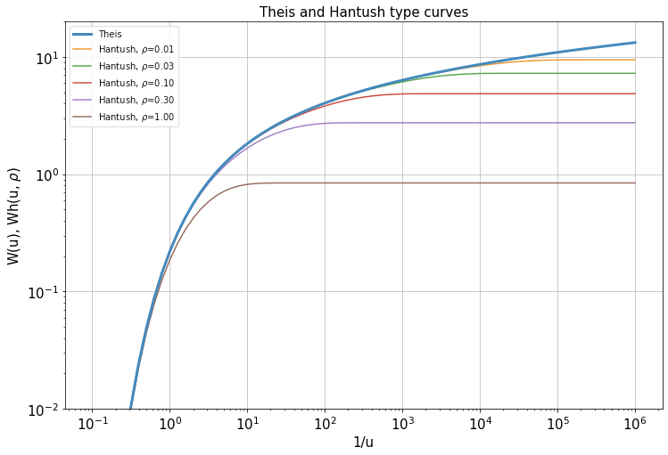
Fig. 7.5 Theis and Hantush type curves
7.4.5.1. Example application
In the past, these type curves have always been used to compute the drawdown. For instance say we want to compute the drawdown at \(r=250\) m from the well after \(t=20\) d of pumping at a rate of \(Q=1200\) m\(^{3}\)/d. The formula is
Let \(kD=600\) m\(^{2}\)/d, \(S=0.2\), \(c=1200\) d, we then have \(\lambda=\sqrt{600\times1200}=850\) m and \(u=\frac{0.2}{4\times600}\frac{r^{2}}{t}=8.3\times10^{-5}\frac{r^{2}}{t}\) then the drawdown at \(r=250\) m after 20 days will follow from \(u=8.3\times10^{-5}\times\frac{250^{2}}{20}=0.259\) and \(\rho=\frac{250}{850}=0.3\) and \(Q/\left(4\pi kD\right)=1200/(4\pi600)=0.159\), so that
The value of \(W_{h}\) can now be read from the type curve for \(r/\lambda=0.3\). But on the horizontal axes we have to use \(1/u=3.86\), hence \(W_{h}\left(\frac{1}{u}=3.86,\frac{r}{\lambda}=0.3\right)\approx0.6\). Hence, the drawdown at 250 m from the well 20 days after pumping started is \(s=0.159\times0.6=0.95\) m.
As demonstrated, these are quite some steps, whereby instead of reading the function value from the type-curves, it may be looked up in tables presented in books like Kruseman and Ridder (1994). Nowadays it is, of course, much easier to implement the functions in a program such as Python (or Excel) and use them. This allows to making graphs that involves many points at once and also to applying superposition easily, which by hand also requires many table look-ups.
7.4.5.2. Unconfined flow approximation by Theis:
Above we simply used the transmissivity \(kD\) without worrying about its change due to the drawdown \(s\) itself. However, we can obtain a somewhat more accurate drawdown in case of a water table aquifer by taking the change of aquifer thickness into account. Theis (1935) himself used the linearization that was described in (7.1). By writing \(2sD\approx h^{2}-D^{2}\) and \(u=\frac{r^{2}S}{4k\overline{h}}\) with \(\overline{h}=0.5\left(h+D\right)\) he obtained as a good approximation to be used for the transient flow to a well in an unconfined aquifer
7.4.5.3. Inflection points in the graphs of the Hantush well functions on half-logarithmic scales (well functions versus log of \(1/u\))
We may further explore the behavior of these two well functions by showing them with a linear vertical scale and a logarithmic horizontal scale see Fig. 7.6. Notice that the vertical axis is reversed (so the drawdown increases downward) to reflect real drawdown. This is not essential. On a half-log scale one sees that with the Theis curves, after some initial time, the drawdown starts increasing linearly with \(1/u\) and, hence, also with time. Each Hantush type curve reaches a maximum value after some time. A characteristic of in these Hantush curves is their inflection point. Each inflection point marks the time at which the Hantush drawdown is exactly half its final equilibrium value. The inflection point is reached for \(u=\frac{\rho}{2}=\frac{r}{2\lambda}\), so \(\mbox{W}_{h}\left(\frac{r}{2\lambda},\frac{r}{\lambda}\right)\). This knowledge can be used to estimate at what time this inflection point is reached at a given distance. Mathematically we have
and, therefore,
The dimension is indeed time. On the other hand, if you have a measured drawdown curve and you recognize with some accuracy the inflection point of the drawdown on linear scale versus \(1/u\) on half-log scales, you may conclude that this point is half-way the final equilibrium value. Also, if your measured drawdown curve shown no sign of inflection towards the horizontal line, then you may conclude that the drawdown is still developing according to the Theis solution and that there is no influence up to that time visible of any leakage through an aquitard above below the aquifer.
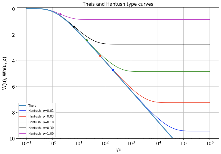
Fig. 7.6 Theis and Hantush function at linear vertical and logarithmic horizontal scale (\(1/u\)) including inflection points for the Hantush well function.
7.4.6. Power approximation of Theis well function
Next to its mathematical integral representation, the Theis well function given in (7.3), the exponential integral can also be written as a power series (e.g. Kruseman and Ridder (1994)):
This \(\gamma\) is the so-called“Euler constant”. It is a fundamental mathematical constant much like \(\pi\) and \(e\), but only less well known.
This power-series form of the Theis well function allows some simplifications, which prove extremely useful in practice, because it simplifies many an analysis and provides a useful characteristic expression like the radius of influence.
Note that for sufficiently small values of \(u\), all the terms with the higher powers and even the term \(u\) will become negligible with respect to \(\ln u\). Take for instance \(u=10^{-4},\,10^{-3},\,10^{-2},\,10^{-1},\,10^{0}\), then \(-\ln u=9.4,\,6.9,\,4.6,\,2.3,\,0\) which should make this clear. Hence, for values of \(u\) less than about \(10^{-1}\), \(-\ln u\) is less than 4% of \(u\). When this is the case, we may approximate the well function to just the first two terms of (7.5):
Hence, for small values of \(u\), that is for very small values of \(r\) or for very large values of \(t\), the Theis drawdown becomes a straight line when plotted versus \(1/u\) or \(t\) or \(t/r^{2}\) on a logarithmic horizontal axis. That is, the drawdown keeps increasing forever by a fixed value per log-cycle of time. Hence the extra drawdown between \(t=\tau\) and \(t=10\tau\) is the same whatever \(\tau\) is, as long as \(u\) is small enough ( \(t\) is large enough). The Theis type-curve on half-log axes already revealed that after some time the drawdown keeps increasing linearly with the log of time, i.e. with by a constant value for every log-cycle of time. But the approximation proves that this must indeed be the case.
7.4.7. Radius of influence
The Theis well function plotted versus \(t\) or \(t/r^{2}\) clearly shows that it takes some time for the drawdown to reach a piezometer at a given distance. Therefore, we may speak of a“radius of influence”, which is dynamic, and indicates to how far from the well the drawdown is perceivable. It is often of practical importance. Clearly, we can define the radius of influence in different ways. For instance, we could say the radius of influence is the distance where the drawdown is 1 cm or, 10 cm or whatever seems appropriate. However, we could, and we do that here, opt for a more general definition. If we inspect the logarithmic approximation of the Theis well function, we see that at any given time, the drawdown is approximately a straight cone when plotted versus distance. Over time, the point of intersection of this straight cone with zero drawdown moves away from the well. It is natural to define the radius of influence to be the distance at which the straight drawdown line intersects the drawdown \(s=0\).
With the log-approximation of the Theis well function, the analysis is straightforward. Starting with the approximation we have
so that for this to be true, the \(\log\) must be 1. So,
With this, we immediately obtain what may we call “the radius of influence”:
It is the radius from the well at which the drawdown is still zero according to the approximate Theis well function. This radius is, therefore, proportional with \(\sqrt{t}\).
It is, obviously, also larger when the transmissivity is larger, causing the well’s influence to spread faster; and it is smaller when the storage coefficient is larger, which reduces the spreading of influence of the well. This simple expression is very practical to estimate how far the influence of a well under the conditions envisioned by Theis reaches as a function of time.
7.4.8. Graphical illustration of the radius of influence
Fig. 7.7 visualizes the radius of influence. The figure shows the drawdown as a function of \(\log(r)\) for different times. The logarithmic approximation is shown as dashed lines. The radius of influence is the distance from the well at which the logarithmic approximation intersects the line of zero-drawdown. These intersections are indicated by the thick dots. Also note that the radius of influence depends on the square root of time. Then, because for the lies in Fig. 7.7 we chose a time series in which each next time doubles the previous value, the distance between the successive radii of influence is the same, as is the distance between successive drawdown curves.
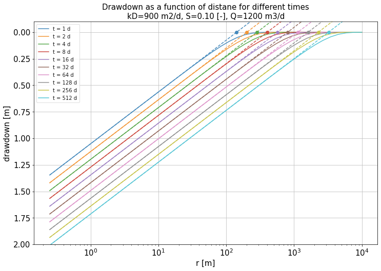
Fig. 7.7 Drawdown versus log of \(r\) for different times. Logarithmic approximation are given as dashed lines. The radius of influence is indicated with a thick dot. Because each next time is twice the previous time, the horizontal distance between the graphs is the same (see formula for the radius of influence).
7.4.9. Relation between the transient Theis drawdown and the well-known Thiem solution for the drawdown in the steady-state situation. Time to reaching steady state.
A steady-state situation will develop after some time when we have any fixed-head boundary at some distance from the well. We can illustrate this using a negative mirror well at some distance \(R\) from our well, which is equivalent to a straight line with a fixed head half-way and perpendicular to the line between the well and its mirror well. Superposition of these two wells yields (using the log-simplification for the Theis solution here for mathematical convenience):
For the drawdown in the well, we have \(r_{1}=r_{w}\), the well’s radius, and \(r_{2}=R\), hence
So if there is a fixed-head boundary somewhere, which in this case we created by putting a mirror well with opposite sign at distance \(R\), this is equivalent to a well at \(r=R/2\) from a fully penetrating river. Adding a mirror well with opposite sign and the same absolute pumping rate, therefore, causes the drawdown to become constant after some time. This is true because the logarithmic approximation will always be valid after sufficiently long times. Also notice that the square under the logarithm leads to \(2\pi kD\) (steady) instead of \(4\pi kD\) (transient) in the numerator of the factor in front of the logarithm. This is always the case in steady-state solutions for wells.
To determine after how much time the steady state is effectively reached is the same as determining after how much time the logarithmic simplification of the well function is valid over the distance \(R\). We may say as shown in before in Power approximation of Theis well function that this is the case when \(u_{t,R}<0.1\). If we have for instance \(kD=600\) m\(^{2}\)/d and \(S=0.2\), and \(R=200\) m, then the time at which the steady state may be set to be effectively reached could be be estimated from
However, the choice of \(u=0.1\) is arbitrary. Another also valid approach is through the argument at the steady state can only be reached after theradius of influence has reached the mirror well. This approach gives
From Fig. 7.7 it may be concluded that the time to reach steady state is, in fact, longer than the time for the radius of influence to reach the mirror well, about 3 times as much seems a better value, which then yields 4.5 days. The best way would be to look at the Theis drawdown on linear scale versus 1/u on log-scale (see Fig. 7.6) to find that the drawdown on this graph as become straight at \(1/u\approx10\) which is the same as \(u\approx0.1\), which is the same as our first estimate in this section and, therefore yields the best estimate for reaching the steady-state situation in this case. In conclusion, because the transition from transient to steady state is continuous, there is not exact point at which the steady state can be said to commence, but it is well possible to give a useful, well informed, quantitative estimate.
7.4.10. Flow at distance \(r\) from the well in the Theis and Hantush situations
7.4.10.1. Theis situation
How much water is released from storage between two distances \(r_{1}\) and \(r_{2}\)? How much is the flow toward the well at distance \(r\)? For such type of questions we need the flow in the aquifer at distance \(r\). For the Theis situation, we can determine this flow analytically, by taking the derivative of the drawdown with respect to \(r\). The derivation goes as follows
so that
With \(u=r^{2}S/\left(4kDt\right)\) it follows that
hence
Using the mathematical expression for the well function, we have
So, finally, we obtain the simple analytical expression
or
This is a very simple relationship between the flow \(Q_{r}\) at distance \(r\) and time \(t\) and the constant extraction \(Q_{0}\) from the well. Because \(u\) is proportional to \(r^{2}\), this ratio diminishes exponentially with the distance from the well. This means that the water comes from storage for say 99% within a given radius from the well. This radius is extending dynamically. Because \(u\) is proportional to \(1/t\), it means that the ratio goes to \(1\) within increasing time over any distance \(r\). This implies that the flow becomes essentially steady, i.e. reaches for instance 99% of the total extraction rate within a given radius after a certain time. Within that radius, the discharge towards the well is essentially equal to the extraction from the well. Hence, over time, the water comes from the storage further and further from the well and the contribution from the zone closer to the well declines to zero over time. Although the drawdown will never become steady state in the Theis situation, the discharge at any fixed distance from the well does become essentially steady state (will approach the well extraction more and more over time).
A constant discharge equal to \(Q_{0}\) within a certain distance implies that the gradients will also become constant within the same distance. This in turn implies that the difference between the drawdowns in observation wells will also become constant and equal to the differences between the heads in these piezometers in the steady-state case, although this steady-state case is never reached. This implies that for sufficiently large times, we can then interpret the transient pumping test like we interpret a steady-state one, but based on the head differences between observation wells. Clearly, this requires the presence of sufficient observation. And, of course, one cannot obtain a storage coefficient from a steady-state analyses.
By way of example, the drawdown and the accompanying ratio \(Q_{r}/Q_{0}\) in (7.6) is shown graphically in Fig. 7.8 firstly as a function of \(t\) for different values of \(r\). Of course, all curves would coincide to a single line if plotted versus \(t/r^{2}\) or \(1/u\) (not shown). The figures 6.9 emphasize the delay occurring with distance from the well (but realize that the time axis is logarithmic). All graphs look the same, except for the delay. Also, notice that once the drawdown becomes a straight line versus log time, the gradients with respect to distance will be constant. This implies that by then, the ratio \(Q_{r}/Q_{0}\) should have asymptotically approached the value of 1. This is easily verified by laying a ruler along the declining branches of the darwdown curves (top chart) and verify from what point in time these curves have become straight lines, and compare this with the extent by which the graph of \(Q_{r}/Q_{0}\) (bottom chart Fig. 7.8) has approached the value of 1.
![[fig:Qr-over-Q0] Top: drawdown. Bottom :math:`Q_{r}/Q_{0}` as a function of :math:`r` for different times and as a function of time for different :math:`r.`\ As before, :math:`Q=1400\,\mathrm{m^{2}/d}`, :math:`kD=600\,\mathrm{m^{2}/d}` and :math:`S=0.1`.](_images/QrOverQ_dd.png)
Fig. 7.8 [fig:Qr-over-Q0] Top: drawdown. Bottom \(Q_{r}/Q_{0}\) as a function of \(r\) for different times and as a function of time for different \(r.\)As before, \(Q=1400\,\mathrm{m^{2}/d}\), \(kD=600\,\mathrm{m^{2}/d}\) and \(S=0.1\).
![[fig:Qr-over-Q0] Top: drawdown. Bottom :math:`Q_{r}/Q_{0}` as a function of :math:`r` for different times and as a function of time for different :math:`r.`\ As before, :math:`Q=1400\,\mathrm{m^{2}/d}`, :math:`kD=600\,\mathrm{m^{2}/d}` and :math:`S=0.1`.](_images/QrOverQ.png)
Fig. 7.9 [fig:Qr-over-Q0] Top: drawdown. Bottom \(Q_{r}/Q_{0}\) as a function of \(r\) for different times and as a function of time for different \(r.\)As before, \(Q=1400\,\mathrm{m^{2}/d}\), \(kD=600\,\mathrm{m^{2}/d}\) and \(S=0.1\).
The total volume that has crossed a radius \(r\) between the times \(t=0\) and \(t=t\) may be computed as
Although this integral does not look difficult, it’s outcome is still nasty. It can be obtained using the integral calculator on the Wolfram site https://www.wolframalpha.com/calculators/integral-calculator/. Although the mathematical solution exists, it is far from trivial, but computing the integral numerically is straightforward usingPython with Numpy and and the quad function from the Python module scipy.integrate.
7.4.10.2. Hantush situation
In the Hantush case, where the drawdowns will become constant over time, the analysis is more difficult. The discharges at any distance is obtained from the derivative with respect to \(r\) from the steady-state drawdown will become constant and equal to (see also Table 7.1 ):
Notice that \(\lim_{r/\lambda\rightarrow0}=1\). The steady state discharge in the Hantush case clearly declines from \(Q_{0}\) at the well to zero at larger distances.
There is not direct analytical expression for the dynamic discharge at \(r\) for the Hantush case. However, it can be computed numerically using the Hantush well function,
which is straightforward using the numerical implementation of the Hantush well function.
7.5. Pumping-test analyses
7.5.1. Introduction
A very important usage of the Theis and Hantush well function is the determination of the aquifer parameters from the drawdowns determined in a pumping test. This section shows such analyses for both the Theis and the Hantush case using artificial data with added noise. The artificial data allow a close comparison between the two situations. The approximate Theis solution (logarithmic) from allows exploiting the behavior of the drawdown on linear scale as a function of the log time and log \(t/r^{2}\). It allows to always compute the transmissivity of the aquifer accurately wherever this drawdown is clearly linear. This is also valid for the Hantush case, because the Hantush drawdown initially follows the Theis drawdown often yielding a nice straight line for early times in well close to the well or from water level measurements inside the well itself.
We will first analyze the pumping test in the Theis situation using the simplified logarithmic well function and then proceed with the classical pumping test analyses on double logarithmic axes. That analysis works the same for the Theis and the Hantush situation. The classic Hantush analysis suffers from the noise in the data. However we overcome this by taking advantage of the mentioned straightforward determination of the transmissivity first, allowing a much better end result.
The considered situation is as shown in Fig. 7.10, which shows a 20 m long well screen penetrating the top 20 m of a 60 m thick aquifer covered by a (semi-)confining layer. Piezometers are present with short screens at two depth, i.e. 10 m and 50 m above the bottom of the aquifer and at 6 distances. The extraction is 2400 m\(^{3}\)/d.
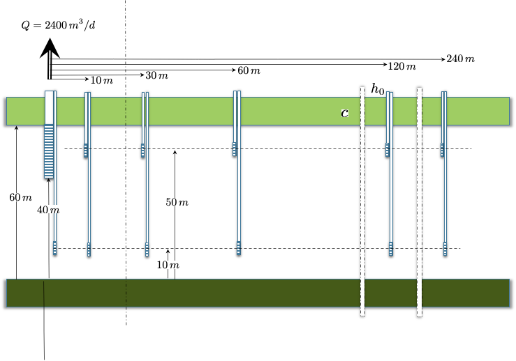
Fig. 7.10 Situation of the pumping test. Partially penetrating well of 20 m length at the top of a 60 m thick aquifer with piezometers at two depths and 6 distances.
7.5.2. Analysis of the pumping test in the Theis situation using the logarithmic approximation of the Theis well function
The logarithmic approximation of the Theis well function that was derived in Power approximation of Theis well function helps enormously with the interpretation of the measured transient drawdowns. We just have to put the drawdown in a graph with the drawdown vertically on a linear axis and the time horizontally on a logarithmic axis. The drawdown in the Theis situation then manifests itself by a linear increase with the log of time. The formula for the Theis drawdown is
Now see what the increase of the drawdown between \(t=\tau\) and \(t=10\tau\) for any time \(\tau\):
and, therefore,
Knowing the well extraction \(Q\) and reading the increase of the drawdown over one log-cycle form the drawdown graph over a portion of the curve where it declines linearly versus log time, then uniquely yields the transmissivity of the aquifer. Hence, it does not matter where the drawdown is measured, in the well itself or in an observation well, as long as we get a linear drawdown per log-cycle, we will thus obtain the aquifer transmissivty. Well clogging, partial penetration (see Partial penetration of well screens ) and any other objections simply play no role here; we only need the drawdown increase per log-cycle where the drawdown increases linearly with log time. This is the simplest an probably the most robust way to determine an aquifer’s transmissivity. And it hold both for the Theis and the Hantush situation.
To what extent is it now also possible to determine the storage coefficient of the aquifer?
In theory it looks easy, but in practice there are complications. Let’s do the theory first and, by the previous analysis we now already know the transmissivity. Given the approximation of the Theis well function, when will the drawdown be zero? The answer is simple, as it is the argument of the logarithm that then must be 1. So we have zero drawdown when
Therefore,
We find the time \(t_{0}\) by extending the straight portion of the drawdown to where it intersects the horizontal line \(s=0\). Now with \(t_{0}\), \(kD\) and the distance to the well \(r\) known, we obtain the storage coefficient from the last expression.
But there are some complications.
When the well screen only partially penetrates the aquifer, the drawdown in piezometers less than about 1.5 \(D\) from the pumping well may suffer from additional drawdown due to the contraction of stream lines near the screen. This effect may even be negative for piezometer screens near the well but well below or above the well screen. The extra drawdown is especially present inside the pumping well if its screen only partially penetrates the aquifer. Therefore, where partial penetration plays a role, the measured drawdown does not reflect the theoretical drawdown that we based our formula on (i.e. the fully penetrating case). And so, simply reading the time where the darwdown line intersects \(s=0\) would not reflect the right value. This can be corrected somewhat by taking partial penetration into account, but only to a limited amount because of unknown vertical conductivity which likely differs from the horizontal one and will vary likely also with depth.
The second complication is that we will not get the correct value if we measure only in the pumping well. Even though we know its radius and even if we know that its screen is fully penetrating the aquifer, the screen may be clogged to some extent. We have no way to estimate this by only measuring the declining head in the well. Therefore, we cannot reasonably expect to obtain a correct value for the time \(t_{0}\) this way. To circumvent complications by clogging of the screen of the pumping well, we must use separate observation wells of which the drawdown is not impacted by potential clogging of their screen nor by partial penetration of the well screen. Therefore, these observation wells should preferably be at least 1.5D away from the well. It is, of course, best to have several observation wells, so that one can verify to what extent each of them yields the same result for \(S\).
In conclusion, use of the logarithmic approximation of the Theis well function is robust and effective to uniquely determine the transmissivity of the aquifer, provided the linear drawdown versus log time increases linearly. However, its use to also determine the storage coefficient is limited in practice due to the fact that at small distances from a partially penetrating well screens the obtained drawdown diverts from the theoretical one. Moreover, inside the pumping well we have an unknown extra drawdown due to its clogging, which makes invalidates the drawdown measured in the well for determination of the storage coefficient even if it were fully penetrating the aquifer. It is best to have more than one separate observation wells at sufficient distance from the pumping well, but in that case we can just as well use other analysis methods.
7.5.2.1. Example
The data for the situation shown in Fig. 7.10 are presented in figure are from a pumping test with extraction \(Q=2400\) m\(^{3}\)/d in a confined aquifer. The data are shown with the drawdown increasing downward. The second chart in the same figure shows the same data versus the log of time. All lines then become straight, declining lines (increasing drawdown) after some initial time, depending on the distance of the piezometer to the well. When this happens, one is sure that the situation that the situation complies with the one that Theis had in mind. As is seen from the lines, all lines finally have the same increase of drawdown per log-cycle. Hence, it does not matter which piezometer or even the water level in the well itself is used to determine the transmissivity. The drawdown per log-cycle is here about 0.49 m as shown by the yellow lines in the middle chart of Fig. 7.11. This yields
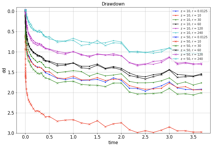
Fig. 7.11 Top: the measurements with the legend denoting the position of the piezometer. Elevation \(z\) relative to bottom of aquifer. \(D=60\) m. Middle: same data but versus logarithm of time. The yellow line is the fitted straight-line through the data for several of the piezometers. The drawdown in the well ( \(z=50\) and \(r=0.25\)) and close to the well fall outside the graph as they are larger than 3 m. Bottom: The same data but now plotted versus \(t/r^{2}\). This makes all drawdown curves collapse onto a single curve except for the piezometers close to the well where partial penetration is important.

Fig. 7.12 Top: the measurements with the legend denoting the position of the piezometer. Elevation \(z\) relative to bottom of aquifer. \(D=60\) m. Middle: same data but versus logarithm of time. The yellow line is the fitted straight-line through the data for several of the piezometers. The drawdown in the well ( \(z=50\) and \(r=0.25\)) and close to the well fall outside the graph as they are larger than 3 m. Bottom: The same data but now plotted versus \(t/r^{2}\). This makes all drawdown curves collapse onto a single curve except for the piezometers close to the well where partial penetration is important.

Fig. 7.13 Top: the measurements with the legend denoting the position of the piezometer. Elevation \(z\) relative to bottom of aquifer. \(D=60\) m. Middle: same data but versus logarithm of time. The yellow line is the fitted straight-line through the data for several of the piezometers. The drawdown in the well ( \(z=50\) and \(r=0.25\)) and close to the well fall outside the graph as they are larger than 3 m. Bottom: The same data but now plotted versus \(t/r^{2}\). This makes all drawdown curves collapse onto a single curve except for the piezometers close to the well where partial penetration is important.
Next, we can read the time at which the extended straight portions of the drawdown graphs intersect the line \(s=0\), zero-drawdown. This is the intersection of the yellow lines in Fig. 7.11 middle chart with the line \(dd=0\). The times for the 4 yellow lines that intersect the line dd=0 in the figure are \(7.5\times10^{-4}\), \(1.5\times10^{-3}\), \(7.0\times10^{-3}\), and \(3.0\times10^{-2}\) days for the orange, green and red lines respectively at 30, 60, 120 and 240 m from the well. Applying
yields \(S=1.7\times10^{-3}\), \(0.8\times10^{-4}\), \(1.0\times10^{-3}\), and \(1.0\times10^{-3}\) respectively. The difference between the first and the rest may be due to the accuracy with which the \(t_{0}\) is read from the graph. It could also result from heterogeneity in the aquifer. However, in this case, a much more important cause will be partial penetration of the well screen due to which the drawdown in piezometers closer than about 1.5D from the well differ from the theoretical value that is valid for a fully penetrating well screen.
The most direct way to verify this is by not plotting the drawdown versus \(\log(t)\) but rather versus \(\log(t/r^{2})\) because this is what the drawdown really depends on. Therefore, plotting the linear drawdown versus \(\log(t/r^{2})\) should force all the drawdown curves to fall on a single one, unless other factors matter, such as partial penetration.
The result is shown in the bottom chart of Fig. 7.11. All the curves for the piezometers that are farther then 60 m away from the well now fall on top of each other. Due to partial penetration, this is not the case for the drawdowns of piezometers that are nearer to the well. The piezometers close to the well (with their screen at 50 m elevation) have a higher than expected drawdown due to concentration of stream lines. The piezometers at the same distance with the screen far below the well face (with screen at 10 m elevation) have a lower than expected drawdown, because the streamlines in this region of the aquifer divert instead of concentrate (see 6.28 ).
The effect of partial penetration is most extreme at the well face. Moreover, the water level in the well itself usually has an extra drawdown even above the effect of partial penetration, which is due to combined clogging of the borehole face and the well face.
If the position of the well screen and the aquifer thickness are known (and also the vertical anisotropy of the aquifer) then is it possible to take partial penetration into account, but this does not work for the drawdown determined in the well itself, because of potential clogging, which requires extra independent information to determine.
7.5.3. Theis and Hantush classic pumping-test analysis
Fig. 7.14 gives the pumping test data for the same aquifer as Fig. 7.11 (middle chart) but now for a semi-confined situation instead of a confined situation, hence we have an Hantush case instead of a Theis case. Also, the same orange dashed lines are plotted that were before used to determine the drawdown per log-cycle in Fig. 7.11. The first thing we see is that now the drawdown will go towards a constant equilibrium value. The blue, red and green lines still yield a correct straight portion that allows computing the drawdown per log-cycle, but the black (\(r=60\) m), purple (\(r=120\) m) and cyan (\(r=240\) m) lines do not. This implies that the trick to determine the transmissivity from the straight increase of the drawdown, i.e. the portion of the drawdown for which the system still behaves like a Theis case, will work, but only for piezometers very close to the well and the well itself. But for larger distances, the previous method fails in the Hantush case.
We’ve seen another property of the Hantush drawdown before, which is the inflection point. If the duration of the pumping test is sufficiently long, so that one can clearly estimate the inflection point, it could be exploited. At the inflection point we have
Although for each inflection point we know \(t/r\), and because we can determine the transmissivity from the drawdown per log-cycle, we are still left with two unknowns in this equation. Therefore, we need a better and more robust interpretation of the pumping test. This is the classical method, which uses the drawdown versus \(t/r^{2}\) on double-logarithmic scales.
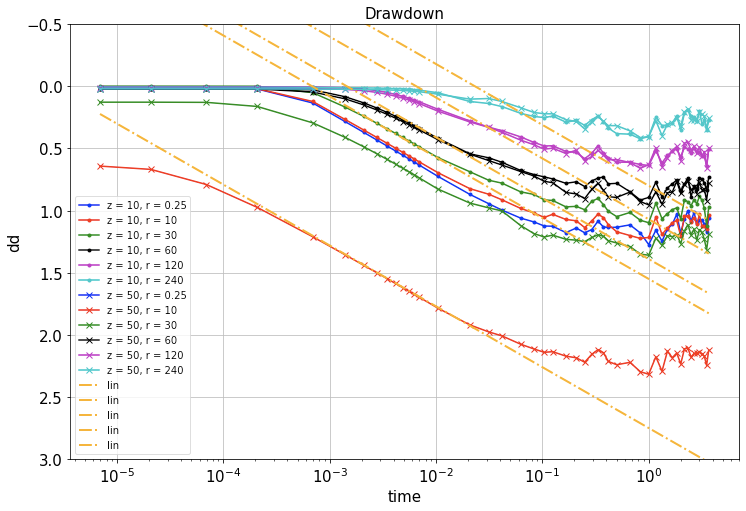
Fig. 7.14 Measurement for the same aquifer and test as in Fig. 7.11 middle graph, but now for a semi-confined aquifer.
Fig. 7.15 shows the drawdown dd [m] on double-log axes. The top chart shows the drawdown versus \(\log t\). The middle chart shows the drawdown versus \(t/r^{2}\). We expect that all lines over the portion that the drawdown still behaves according to the Theis case would fall on one single line, while at later times the lines will deviate from the Theis curve as they approach the Hantush equilibrium. The graph shows that this only works for piezometers further away from the well, here for those least 60 m from the well. This is clear from the curves, which show that at distances larger than 60 m the drawdown in the to and the bottom of the aquifer are the same (See lines with the same color in the charts). The reason is, of course, the impact of partial penetration on the drawdown. Due to partial penetration, the piezometers at 50 m above the base of the aquifer, opposite the well face (at 40-60 m) over-estimate the drawdown. On the other hand, the piezometers at 10 m above the bottom of the aquifer, i.e. far below the bottom of the well, under-estimate the drawdown. The closer to the well, the more extreme this over- en underestimation is. The drawdown in the well itself (almost 10 m!) is further increased by clogging. For our interpretation we have to leave these piezometers out. Therefore we’ll limit our analysis to the piezometers at 60, 120 and 240 m from the well. Their drawdowns are shown in the bottom chart of Fig. 7.15.
![Top: Drawdown :math:`dd` [m] (upward) versus :math:`t` [d] on double-log axes. Middle: drawdown [m] (upward) versus :math:`t/r^{2}` [d/m :math:`^{2}`\ ] on double-log axes. Bottom: same as middle chart, but leaving out the piezometers closer than 60 m, that are definitely influenced by partial penetration, while the drawdown in the well itself is also likely further enhanced by clogging. The bottom chart is also zoomed in on the portion with the larger drawdowns, so that they are less impacted by noise in the measurements.](_images/pptest_hantush_doublelog1.png)
Fig. 7.15 Top: Drawdown \(dd\) [m] (upward) versus \(t\) [d] on double-log axes. Middle: drawdown [m] (upward) versus \(t/r^{2}\) [d/m \(^{2}\)] on double-log axes. Bottom: same as middle chart, but leaving out the piezometers closer than 60 m, that are definitely influenced by partial penetration, while the drawdown in the well itself is also likely further enhanced by clogging. The bottom chart is also zoomed in on the portion with the larger drawdowns, so that they are less impacted by noise in the measurements.
![Top: Drawdown :math:`dd` [m] (upward) versus :math:`t` [d] on double-log axes. Middle: drawdown [m] (upward) versus :math:`t/r^{2}` [d/m :math:`^{2}`\ ] on double-log axes. Bottom: same as middle chart, but leaving out the piezometers closer than 60 m, that are definitely influenced by partial penetration, while the drawdown in the well itself is also likely further enhanced by clogging. The bottom chart is also zoomed in on the portion with the larger drawdowns, so that they are less impacted by noise in the measurements.](_images/pptest_hantush_doublelog2.png)
Fig. 7.16 Top: Drawdown \(dd\) [m] (upward) versus \(t\) [d] on double-log axes. Middle: drawdown [m] (upward) versus \(t/r^{2}\) [d/m \(^{2}\)] on double-log axes. Bottom: same as middle chart, but leaving out the piezometers closer than 60 m, that are definitely influenced by partial penetration, while the drawdown in the well itself is also likely further enhanced by clogging. The bottom chart is also zoomed in on the portion with the larger drawdowns, so that they are less impacted by noise in the measurements.
![Top: Drawdown :math:`dd` [m] (upward) versus :math:`t` [d] on double-log axes. Middle: drawdown [m] (upward) versus :math:`t/r^{2}` [d/m :math:`^{2}`\ ] on double-log axes. Bottom: same as middle chart, but leaving out the piezometers closer than 60 m, that are definitely influenced by partial penetration, while the drawdown in the well itself is also likely further enhanced by clogging. The bottom chart is also zoomed in on the portion with the larger drawdowns, so that they are less impacted by noise in the measurements.](_images/pptest_hantush_doublelog3.png)
Fig. 7.17 Top: Drawdown \(dd\) [m] (upward) versus \(t\) [d] on double-log axes. Middle: drawdown [m] (upward) versus \(t/r^{2}\) [d/m \(^{2}\)] on double-log axes. Bottom: same as middle chart, but leaving out the piezometers closer than 60 m, that are definitely influenced by partial penetration, while the drawdown in the well itself is also likely further enhanced by clogging. The bottom chart is also zoomed in on the portion with the larger drawdowns, so that they are less impacted by noise in the measurements.
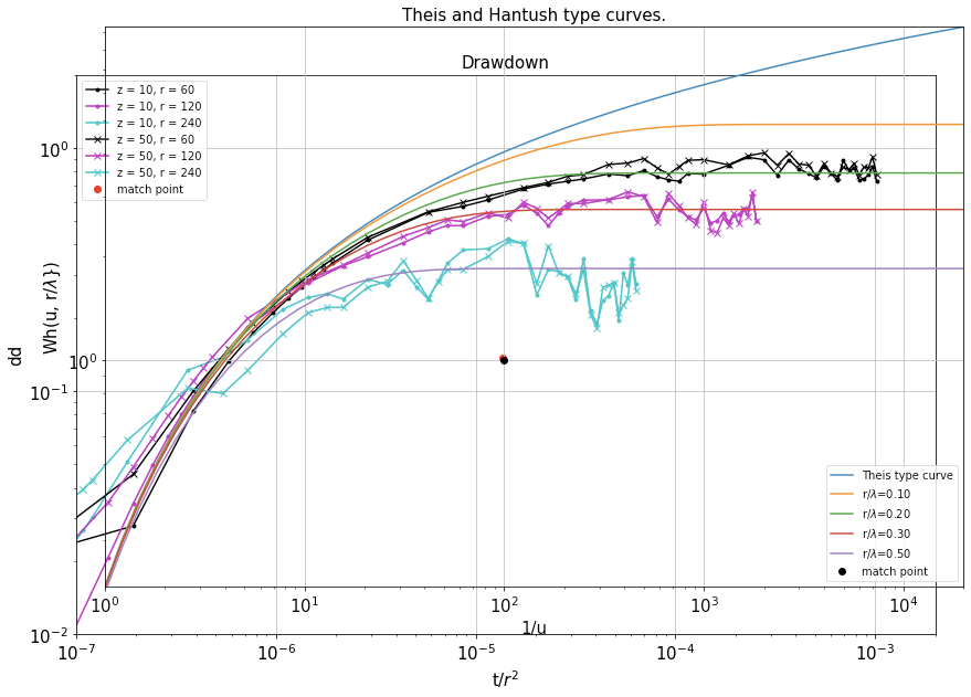
Fig. 7.18 Two overlapping sheets. One with the measured drawdown \(s\) versus \(t/r^{2}\) and the other, separate sheet, with the Theis and Hantush well function versus \(1/u\). Both charts are on double log scales and the width of the log-cycles are the same. The chart with the Theis and Hantush type curves have been shifted over the measurements until the best fit was reached by eye. Then the match point was chosen to be used in the analyses to determine the transmissivity and the storage coefficient and, finally, the resistance of the aquitard.
To interpret the pumping test, we will overlay the measurements with the Hantush type-curves plotted on a different sheet of paper but making sure that the width of the log-cycles both vertically and horizontally are the same as of the double-log graph of the measurements, where drawdown \(dd\) was plotted against \(t/r^{2}\). This is shown in Fig. 7.18.
Because we use double log paper, the type curves should have exactly the same shape as the measurements. The reason is that the drawdown is obtained by multiplying the well function by a constant (i.e. the as yet unknown value of \(Q/\left(4\pi kD\right)\), and multiplying by a constant is done by shifting by a constant on log-scale. Further, because \(1/u=\frac{4kD}{S}\times\frac{t}{r^{2}}\), the horizontal axis of the graph of the measurements and that of the type-curves also differ by a factor (the as yet unknown value of \(\frac{4kD}{S}\). On log-scale this implies a horizontal shift of the two axes relative to each other. But in any case, the shape of the measurement curves should be exactly that of the type curves.
Therefore, when we have the measurements and the type curves on two separate sheets of paper such that the size of each log-cycle both horizontally and vertically are the same in both graphics, then we can overlay them and shift them with respect to each other such that the measurements and the type-curves match as well as possible.
Once we have this, we choose an arbitrary point (just prick a pin at that point through both sheets of paper) and call it the match point (I chose the big dot in Fig. 7.18). Then read the value of \(s\) and \(t/r^{2}\) for the match point from the measurement sheet. This yields \(t/r^{2}=1.37\times10^{-5}\) and \(s=0.137\). Next, read the value of \(Wh\) and \(1/u\) for the match point from the sheet with the type-curves. This yields \(1/u=100\) and \(\mbox{Wh}=1\).
With these data compute the transmissivity and the storage coefficient.
First we focus on the vertical axes of the two charts using the values of the match point, for which we obtain:
Next, we focus on the horizontal axis, for which we have:
The resistance of the aquitard then follows from which line of the Hantush type curves actually fits the measurements.
For \(r=60\) m we find the type curve for \(r/\lambda=0.2\), for \(r=120\) m we it is the type curve for \(r/\lambda=0.3\) and for \(r=240\) m it is \(r/\lambda=0.5\). Hence, the \(\lambda\)-values that we find are \(60/0.2=300\) m, \(120/0.3\) = 400 m and \(240/0.5\)=480 m. So it must be around 400 m. The aquitard resistance then becomes \(c=\lambda^{2}/kD=400^{2}/2800=60\) d.
This is the classical pumping test analysis. It works the same for Theis and Hantush. However, for Hantush we will also find the values of \(r/\lambda\) and, therefore, of \(\lambda\), which in turn yields the resistance of the aquitard when we have already determined the transmissivity of the aquifer.
7.5.3.1. Can we improve the accuracy?
Yet in this case, the interpretation does not seem to be very accurate as the three \(\lambda\) values are not very consistent. This is a consequence of the noise in the data. Can we do better? Remember that we may always determine the transmissivity from the drawdown per log-cycle, which is independent of partial penetration. We only need drawdown that has a sufficiently long straight portion on half-log scale. It is likely that the drawdowns close to the well and that inside the well itself will exhibit such an opportunity. Fig. 7.14 shows that this is indeed the case for the drawdown at \(z=50\), \(r=10\), which yields a drawdown per log-cycle of 0.49 m and so we have
With the transmissivity known accurately, we also know the vertical shift of the two vertical axes required to let the Hantush-type curves overlap the data. This would be
where \(Q/\left(4\pi kD\right)=2400/(4\pi900)=0.212\). Therefore, we obtain
With respect to the horizontal axes we have
In which \(S\) is the only remaining unknown. Hence, by changing \(S\) by trial and error in (7.7), we can now shift the computed Theis drawdown horizontally such that it matches the data as well as possible. The results are shown in Fig. 7.19, top chart. The computed Theis line that best fits the data is make thicker an dashed red. With the transmissivity \(kD=900\) m\(^{2}\)/d and \(S=0.008\) now secured, we can overlap the measurements with the lines computed using the Hantush well function for a suitable set of values for \(\rho=r/\lambda\). The results are shown in Fig. 7.19, bottom chart. This final chart allows us to select the best values for \(r/\lambda\) for the three observation distances. We thus find \(\rho\approx0.17\) for \(r=60\) m, \(\rho\approx0.32\) for \(r=120\) m and \(r\approx0.7\) for \(r=240\) m. And so we have three approximations for \(\lambda\)= \(r/\rho\) namely \(60/0.17=353\), \(120/0.32=375\) and \(240/0.7=343\) m, hence, consistent results with an average value of \(\lambda\approx360\) m from which we obtain \(c=\lambda^{2}/kD=360^{2}/900=145\) m.
In conclusion, we have interpreted the pumping test in a classical fashion, making use of the fact that the type curves and the measurements must have the exact same form on double log axes, under the conditions that there is no effect of partial penetration. We have experienced that the results may be less exact due to the presence of noise in the data resulting from phenomena like weather and barometer pressure fluctuations that have nothing to do with our pumping test, but can not be avoided in practice when pumping tests last for several days or weeks. Despite the difficulties resulting from this noise, we were able to take advantage of the universal fact that the transmissivity can be obtained uniquely and accurately from the straight portion of the drawdown when plotted versus the log \(t\), irrespective of partial penetration or even clogging of the well in case we measure the water level inside the well. This is also due to the fact that even in a semi-confined Hantush situation, the observation points close to the well still show a consistent Theis behavior at early times, allowing to extract a straight portion of the drawdown curves versus log \(t\) . With the transmissivity thus known accurately, we know the vertical shift of the measurement chart relative to the chart with the type curves, so that the charts only have to be shifted horizontally to find the best fit. This particular exercise was done in the computer, by plotting the Theis drawdown curves for a range of storage coefficients directly on the measurement chart, which allowed us to pick the one that best fits the data. With then both the transmissivity and the storage coefficient fixed, we could overlap the measurements with a bundle of Hantush computed drawdowns, for a range of values for \(\rho=\frac{r}{\lambda}\). This allowed us to pick the best fitting \(r/\lambda\) for the measurements of the piezometers at different larger distances from the well. As a result, we obtained an \(r/\lambda\) value for each of the three piezometer distances, which in turn yielded three mutually consistent values for \(\lambda\). The average of these, combined with the transmissivty finally gave us the hydraulic resistance \(c\) of the aquitard. The final results are accurate and fully consistent with the data.

Fig. 7.19 Top: The measured and computed Theis drawdowns as a function of \(t/r^{2}\) for multiple values of the storage coefficient \(S\). The best-fitting Theis curve is the dashed red line, which is for \(S=0.008\). Bottom: The curves with the measurements overlapped with the Hantush curves for the best storage coefficient. Note that the thicker drawn blue line in the bottom chart (Theis drawdown) is the same as the dashed thick red line in the top chart.
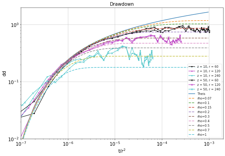
Fig. 7.20 Top: The measured and computed Theis drawdowns as a function of \(t/r^{2}\) for multiple values of the storage coefficient \(S\). The best-fitting Theis curve is the dashed red line, which is for \(S=0.008\). Bottom: The curves with the measurements overlapped with the Hantush curves for the best storage coefficient. Note that the thicker drawn blue line in the bottom chart (Theis drawdown) is the same as the dashed thick red line in the top chart.
7.5.4. Exercises
The book Kruseman and Ridder (1994) describes a pumping test “Oude Korendijk” and provides the data. Interpret that test.
An unconfined aquifer has a transmissivity of \(kD=500\) m\(^{2}\)/d and a specific yield of \(S_{y}=0.15\) and is situated above an impervious base. Groundwater is extracted during 2 weeks. During the first 10 days, the extraction rate is \(Q=1000\) m\(^{3}\)/d; during the last 4 days, the abstraction is \(Q=3000\) m\(^{3}\)/d. What is the drawdown \(s\) at the end of this 2-week period at a distance o \(r=80\) m from the well?
A square building pit with sides of \(L=50\) m needs its construction floor at 7 m below ground surface to be put dry. The water table is initially at 4 m below ground surface. The aquifer is unconfined with its bottom at 50 m below ground surface. The hydraulic conductivity is estimated at \(k=20\) m/d and the specific yield is \(S_{y}=0.25\). The construction need to start in 4 weeks, so the floor of the building pit must by dry by then. It takes one week to install a well at each corner of the building pit. What capacity \(Q\) must each these wells have to realize a groundwater level that is 50 cm below the building-pit floor in 4 weeks?
The Nubian sandstone aquifer is the world’s largest known aquifer system (See Wikipedia and Fig. 7.21). It measures 2 million km\(^{2}\), covering large parts of NW Sudan, NE Chad, SE Libya and most of Egypt. It contains an estimated amount of 150000 km\(^{3}\) of fossil groundwater. It may be considered confined with a transmissivity of 600 m\(^{2}\)/d. Libya under Gaddafi created the so-called Great Man-Made River Project. It began extracting 2.4 km \(^{3}\)/year (6.6 million m\(^{3}\)/d or 275000 m\(^{3}\)/h or 76 \(\text{m}^{3}/\text{s}\) in the mid 1990. The wells of Kufra can be easily found on Google Earth; they are 400 km away from the Egyptian border. Assume that the wells in Kufra extract 15 m\(^{3}\)/s from the Nubian aquifer. If continued, how will the drawdown in the Nubian aquifer develop at the border between Egypt and Libya?

Fig. 7.21 Picture of the GMMR project in Libya
Groundwater is extracted from an unconfined aquifer to irrigate crops by means of a pivot, i.e. a well connected to an irrigation frame that slowly turn around the well. This pivot irrigates a disc of a surface are of 50 ha. 50% of the irrigated waters is consumed by the crop and hence evaporated by it; the remaining 50% is water that returns to the aquifer. A crop consumes a water volume equivalent to a layer of 75 cm over the area served. Two crops can be harvested each year. What is the required pumping capacity of the well and how will the groundwater head below the pivot develop? To answer this question, compute the drawdown over time at the following distances from the well a) 0.2 m (=inside the well, required to see if the well could fall dry in the near future), b) at the edge of the irrigated 50ha circular area served by the well, c) at 2 and 5 times this radius to estimate its impact on neighboring wells.
An area in Morocco is irrigated by means of drainage tunnels (qanats, or khettarras, see Wikipedia, see Fig. 7.22). The water to the aquifer is rainwater that was captured in the nearby hills and mountains. The general groundwater flow away from the foot of the mountains causes a gradient of the natural groundwater, which is exploited by the drainage tunnels. These tunnels run from their downstream outlet in the villages with a small upward gradient towards the foot of the mountains, where they intersect the water table, so that groundwater will drain and flow towards the village through these tunnels. Assume that the average drawdown caused by these tunnels is 2 m. A developer intends develop a farm to grow crops in a new area nearby and wants to install wells for irrigation. The area to be irrigated is 50 ha and the required net consumption is 0.75 m/year, hence a required year-average extraction of \(0.75\times50000/365=1030\mathrm{m^{3}/y}\). What will be the impact of the extraction wells on the existing khettaras? Take into consideration that the aquifer at the foot of the mountains is closed and that its open to infinity away from these mountains. Assume the specific yield is 20% and the transmissivity is \(500\,\mathrm{m^{2}/d}\). Realize that there are no fixed-head boundaries, i.e. the groundwater will always be in dynamic equilibrium. So the effect of the new development will also be transient. Compute the drawdown that it causes over time in the drainage area of the qanats. Realize that the mountain face works as a groundwater barrier.

Fig. 7.22 Qanats new mountain area with village and projected new development in desert
Som thoughts about the problem stated above. It may not seem immediately obvious to provide an answer with the simple tools of this course. But we can give it a try. We can compute the transient drawdown by the new well compute its effect near the foot of the mountains. With this, we can compute the drawdown everywhere, and therefore, also at every point of the qanats where they tap the groundwater, which is in the qanat drainage area. We may assume that the yield of the qanats is proportional to the drawdown they cause, which was 2 m. When we subtract the drawdown of the new well at the khettaras from that of the khettaras themselves, we have at least an estimate of the impact. A difficulty arises only from the integration of the drawdown impact along each khettara. However, we can just take the drawdown that the center of their tapping length as an approximation.
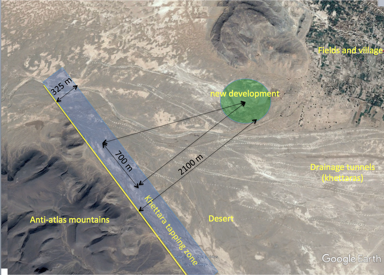
Fig. 7.23 So-called Khettaras (better known by the Iranian word qanats = drainage tunnels) to the west of Erfoud in Morocco draining groundwater from the foot of the Anti-Atlas mountains at the left to the fields and villages at the right (coordinates lat 31.506, lon -4.484). The width of the figure is 5600 m.
In the Mid-West of the United States, rights for water extraction from a creek have been fixed since the nineteenth century. A new development wants to circumvent those rights by using groundwater. Due to the distance from the creek, i.e. 800 m, no impact on the creeks discharge is expected. But will this be true? The aquifer is unconfined with a specific yield of 0.24, a depth of 60 m and a conductivity of about 25 m/d. Compute whether there is an impact of the extraction by the new farmer who intends to extract a year-round average of 1000 m\(^{3}\)/d. If so, how will this impact grow over time? When will it reach its maximum? What will be the maximum impact of this extraction?
7.5.5. Superposition in time
We will illustrate superposition in time for the Theis situation, however, it works exactly the same for the Hantush case.
A well may be switched on and off at will. The effect of this switching can be taken into account by superposition. For instance, a well that has been pumping for a time \(\Delta t_{i}\) since \(t=0\), after which it is switched off, can be viewed as two wells that pump continuously. The first starts at \(t_{0}=0\) with extraction \(Q_{0}\) and the second at \(t=t_{0}+\Delta t_{i}\) with extraction \(-Q_{0}\). This way, the net extraction will be zero for \(t>t_{0}+\Delta t\). This superposition can be applied with a large number of changes of the flow rate at arbitrary times. The problem may only be that after many such changes one needs to carry on a large number of“wells” at the location of the real well to compute the current state. This is merely a computational burden, one that can be effectively dealt with through application of convolution, explained elsewhere in this syllabus.
Hence, we have for a well that switches on at \(t=t_{0}\) and then switches off at \(t=t_{0}+\Delta t\)
where the second term is omitted al long as \(t<t_{0}+\Delta t\).
To deal with a well with varying extraction, we subdivide time in episodes during which the extraction from the well may be considered sufficiently constant. In this superposition we start a new well at the same position each time the flow rate changes. We let this new well extract the difference between the new rate and that of the previous well.
For example, let the flow rate change at rate-change times \(t_{0},t_{1},t_{2},t_{3},\dots\) after which the flow rate is \(Q_{0},Q_{1},Q_{2},Q_{3},\dots\), respectively. We can simulate the heads by starting a new well at each of these rate-change times with extraction
because after \(t_{0}\) the total extraction is \(Q_{0}\), after \(t_{1}\) ti is \(Q_{0}+Q_{1}-Q_{0}=Q_{1}\), after \(t_{2}\) it is \(Q_{1}+Q_{2}-Q_{1}=Q_{2}\) etc. Applying superposition then yields
To check, take any time, say \(t_{i}\) so that all wells \(0\rightarrow i\) are active and add all the flows for these well to get \(Q_{i}\) which is the true total extraction at that time.
With this in mind, superposition for an arbitrarily varying well becomes straightforward. Just assemble the list \(t_{i}\) and \(Q_{i}\) for \(i=0\rightarrow n\). The flow of the wells to be switched on at times \(t_{i}\) is then simple the difference of consecutive flows. Let’s call these flow changes \(\Delta Q\), then \(\Delta Q_{i}=Q_{i}-Q_{i-1}\) for \(i>0\) and \(\Delta Q_{0}=Q_{0}\)
Example:
Consider an aquifer of infinite lateral extend with \(kD=600\,\mathrm{m^{2}/d}\) and \(S_{y}=0.1\). If well extracts at the following flows during according to the middle picture in Fig. 7.24. The drawdown at 5 different distances (see title of top picture) are computed by superposition and are shown the top picture. The distance \(r=0.01\) represents the well face. The lower picture of Fig. 7.24 illustrates the superposition better for the piezometer at 50 m distance. It shows not only the result of the superposition, but also the contribution of each individual change of the well rate.

Fig. 7.24 Superposition in time (for data given in the text example). \(kD=600\) \(m^{2}/d\), \(S=0.1\).
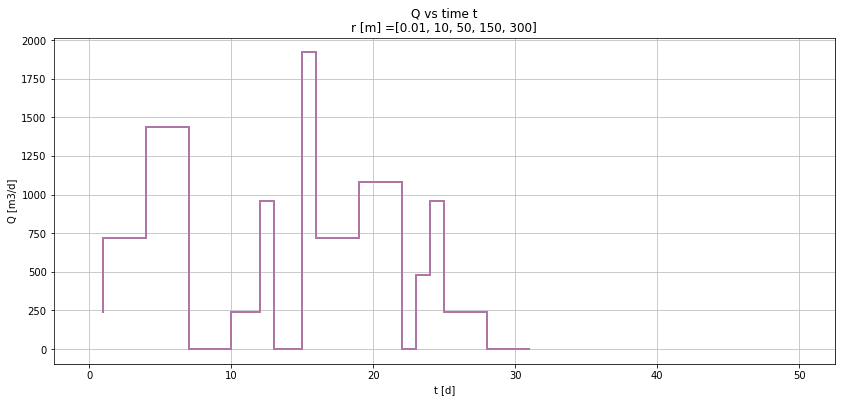
Fig. 7.25 Superposition in time (for data given in the text example). \(kD=600\) \(m^{2}/d\), \(S=0.1\).
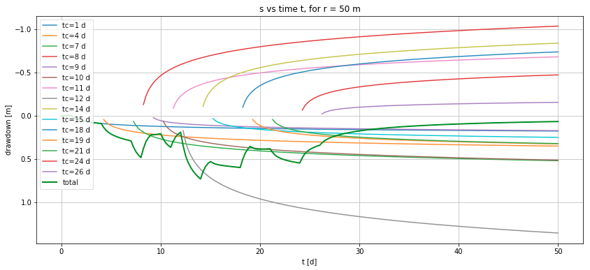
Fig. 7.26 Superposition in time (for data given in the text example). \(kD=600\) \(m^{2}/d\), \(S=0.1\).
Of course, it is rather straightforward to carry out superposition with many well simultaneously, where each of them has a flow rate that varies independently of the other wells, and compute the resulting varying head or drawdown at an arbitrary location. And if we do this for many location simultaneously, we can show the the head contours in an entire region fluctuating under the influence of many wells of which each extracts at it’s own will.
7.5.6. Superposition in space
The contributions of an arbitrary number of pumping wells can be added together, because the underlying partial differential equation is linear. Therefore, superposition works in space as well as in time. One can have an arbitrary number of wells that are pumping arbitrary amounts of water, and compute the drawdown at any number of arbitrary points simultaneously by superposition of the ensemble of wells, while per well the superposition in time is done as explained in the previous section. Because superposition is valid, the drawdown can be superimposed on the ambient groundwater head to get the real head in the aquifer.
Example: Consider an area with are four wells. Each well each is constructed and starts exactly one year after the previous well. The four wells are placed on a square area with sides of 1 km. The order in which they are constructed is NW, NE, SE SW. The extraction is 600 m\(^{3}\)/d at from each well. The transmissivity is \(kD=600\) m\(^{2}\)/d and the specific yield is \(S_{y}=0.24\). Visualize the drawdown in the center of the area between these wells as a function of time for a period of 10 years. Show spatial snapshots of the drawdown at times \(t=[0.5,1.5,2.5,3.5,4.5]\) years after the start of the first extraction well.
Fig. 7.27 shows the result of superposition in time for the point in the center of the square with the four wells at the corners. This is the same as in the previous example. Both the total result and the effect of each individual well are shown. It is practical in this case, to work in years and convert the transmissivity and the extraction to years instead of days.
For the spatial snapshot we compute the drawdowns in a dense-enough spacial grid to allow contouring of the drawdown at a specific point in time. The grid used is 10 m spacing between -1000 and +1000 m for both the \(x\) and the \(y\) axis. With these coordinates, the distance is computed to each of the wells. The distance from the grid points to one well is already 160000 points (this requires Python, Excel can’t hardy handle this). To prevent division by zero make sure the the minimum distance is \(r_{w}\), the well radius. Zero distance occurs of a grid point happens to coincided with the position of a well.
Finally, for each of the four required snapshot times, add the contribution of each of the four wells and for each well use the time since the extraction from that well started. The last step is to contour the results as presented in Fig. 7.27. The figure uses the same contour lines in all four snapshots, but the values are not indicated in the figure . This, could, however, been done by using full colors and placing a color bar next to each figure . Each snapshot is taken 0.5 years after the previous well started.
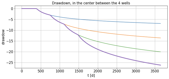
Fig. 7.27 Computed drawdown for the example in the center between the four wells (thick black line) and at well #1 (thick dashed purple line)
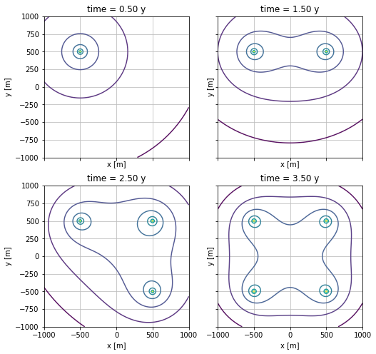
Fig. 7.28 Snapshot of drawdown after 50 years of pumping; the colors match the drawdown shown in Fig. 7.27.
7.5.6.1. Exercise:
In Egypt, an investments to grow fruits have been made in the desert along the motorway between Cairo and Alexandria. Imagine the enterprise’s premises to be 2 km wide having 500 ha of cropped area, that is 2 km along the road by 250 m perpendicular to the road. The crop requires 1 m of water per year irrigation. Four wells are used arranged parallel to the road. They all have their screen from -50 to -100 m. What will be the drawdown in the middle two wells after 1 month, 1 year, 10 years and 50 years. Also compute what will be the drawdown at the neighbor farms 2, 4, 6, 8 and 10 km away. Finally, what would be the drawdown in the center wells if these neighbors up to 10 km away on both sides would pump at the same rate? The transmissivity of the aquifer is \(kD=2000\) m\(^{2}\)/d, the specific yield is \(S_{y}=0.24\), the depth of the aquifer is 240 m and the distance below ground surface was 40 m initially. (See also the paragraph on partial penetration).
7.5.7. Questions
What groundwater situations are solved by Theis? What are the conditions for the underlying groundwater system, and the initial and boundary conditions so that Theis applies?
Why do we prefer drawing the Theis well function (type curve) on a double log graph using \(1/u\) instead of \(u\) on the horizontal axis?
Explain how we can interpret a pumping test in a confined aquifer based on the Theis type curve on a double log graph?
What is the preferred variable to use on the horizontal axis when plotting the drawdown data coming from different observation wells, and why?
What is the physical meaning of the partial differential equation on which the Theis solution is based?
Is there a final steady state situation that matches the Theis solution?
How is the outcome \(h^{2}-H^{2}=\frac{Q}{2\pi k}\mbox{W}\left(u\right)\) related to that of a confined situation, \(h-H=\frac{Q}{4\pi kH}\mbox{W}\left(u\right)\)?
How can you determine \(u\) as a ratio of time \(t\) and a characteristic time \(T\)?
Show how you can simplify the Theis well function for small values of \(u\).
What is the general shape of the Theis drawdown curve on linear vertical and logarithmic horizontal scale?
What part of this general shape is covered by the simplification of the Theis drawdown?
Explain the shape of the drawdown versus distance using the simplified Theis well function \(s=Q/\left(4\pi kD\right)\ln\left(2.25kDt/\left(r^{2}S\right)\right)\)?.
Express this simplified function in terms of the ratio of distance and a characteristic distance for a chosen fixed time.
Explain the radius of influence mathematically using the simplified Theis well function.
What is the drawdown per \(\log_{10}\)-cycle of time? Show this using the simplified formula?
What is the mathematical standard function that is equivalent to the Theis well function?
Given the Theis well function as a power series, (7.5), show the relation between to consecutive terms.
How would you use the Theis well function to compute the drawdown of a well in an aquifer of infinite extent to compute the transient drawdown due to a well at a given distance from a river that fully penetrates the aquifer without entry resistance?
Write down mathematically the superposition in time of a well that changes the extraction in steps from time to time.
How would you compute the drawdown due to a well in an aquifer bounded by two parallel fully penetrating canals in direct contact with the aquifer? The canals are a distance \(L\) apart and the well is at a distance \(l\) from one of them.
Does the situation posed in the previous question result in a steady-state situation on the long run? Explain your answer.
Assume that Libya’s large pumping station in Kufra (E 24.149163°, N 23.392326°), with wells in the Nubian sandstone at 162 km from the Egypt’s border extracted 1 million \(\mathrm{m^{3}/d}\) starting in 2000. How long would it take for the drawdown to influence the head at the border of Egypt? Assume \(kD=600\,\mathrm{m^{2}/d}\), \(S=0.005\). What would be the drawdown at Kufra after 10 and 50 years. What would be the drawdown at the Egyptian border after 10 and 50 years. For the Kufra well field use an effective well radius of 10 km. (have a look at the site on the given coordinates in Google Earth).
If the conductivity of the Nubian sandstone measured in the lab at 20 \(^{o}\)C would be \(k=10\) m/d. What would the conductivity be in the Nubian sandstone at 600 m depth where the water temperature is 50 \(^{o}\)C? And so what conductivity should you use in your computations?
The water table in a building pit of \(50\times50\) m has to be lowered by 5 m. For this, wells are placed at the corners of the pit building pit. The transmissivity \(kD=1000\,\mathrm{m^{2}/d}\) and the specific yield is \(S_{y}=0.2\). Compute the necessary extraction if the water level in the center has to reach this objective (5 m drawdown) within two weeks of pumping. After reaching the necessary drawdown, the drawdown has to be maintained for 6 months. Compute the necessary extraction such that the objective is fulfilled. How much may the extraction be reduced after two weeks, to maintain the desired drawdown, such that the objective is met after 6 months? Hint. If you have code this situation in Python and you use one rate per month, you can just tweak the extraction values until the drawdown matches the requirements.
A well is drilled in an unconfined aquifer to secure water for a refugee camp in Jordan. The transmissivity is small, only \(250\,\mathrm{m^{2}/d}\), and the storage coefficient also is modest with \(S_{y}=0.005\). The water table is at 50 m below ground surface. What is the necessary depth of the screen so that the well will still yield the required demand of \(\mathrm{m^{3}/d}\) after 10 years?
7.6. Partial penetration of well screens
More often than not, well screens only partially penetrate the exploited aquifer because aquifers may be much thicker than the screen length that is needed to produce the required amount of water. Limiting well depth saves money for the owner, although at the cost of some extra pumping energy, because of the extra head loss due to the fact that the streamlines of the water flowing towards the well have to concentrate near the screen, which causes it to accelerate, and higher velocities entail greater losses of energy.
7.6.1. Huisman’s method

Fig. 7.29 Partially penetrating wells
The flow due to only the fact that the screen is partially penetrating can be superimposed on the ideal situation in which the streamlines are all horizontal and parallel with respect to top and bottom of the aquifer when towards a fully penetrating screen, for which the standard groundwater-well formulas were all derived. There are at least two ways to deal with it; both lead to an extra drawdown that must be added to the drawdown obtained with the standard formula.
The first method is to compute the effect of partial penetration based on the exact solution for the effect, which was derived for a confined aquifer by Hantush (see Kruseman and Ridder (1994)). The other is a method developed by Huisman (1972), which summarizes the first method by a simple relation for the extra head loss in the well itself. He writes (p130):“With a random position of the well screen as shown in Fig. 7.30 (left), the additional drawdown at the well face is given by
with \(\alpha\) a function of the amount of penetration \(p=h/D\) and the amount of eccentricity \(e=\delta/D\). The value of \(\alpha\) as a function of these parameters is given in Table 7.2.
p \(\downarrow\) e\(\,\rightarrow\) |
0 |
0.05 |
0.1 |
0.15 |
0.2 |
0.25 |
0.3 |
0.35 |
0.4 |
0.45 |
|---|---|---|---|---|---|---|---|---|---|---|
0.1 |
0.54 |
0.54 |
0.55 |
0.55 |
0.56 |
0.57 |
0.59 |
0.61 |
0.67 |
1.09 |
0.2 |
0.44 |
0.44 |
0.45 |
0.46 |
0.47 |
0.49 |
0.52 |
0.59 |
0.89 |
|
0.3 |
0.37 |
0.37 |
0.38 |
0.39 |
0.41 |
0.43 |
0.50 |
0.74 |
||
0.4 |
0.31 |
0.31 |
0.32 |
0.34 |
0.36 |
0.42 |
0.62 |
|||
0.5 |
0.25 |
0.26 |
0.27 |
0.29 |
0.34 |
0.51 |
||||
0.6 |
0.21 |
0.21 |
0.23 |
0.27 |
0.41 |
|||||
0.7 |
0.16 |
0.17 |
0.20 |
0.32 |
||||||
0.8 |
0.11 |
0.13 |
0.22 |
|||||||
0.9 |
0.06 |
0.12 |
The screen in the center of Fig. 7.30 shows the position that is most usual. This simplifies the formula, at least for penetrations larger than 20%, yielding:
The partial penetration for the right-most screen in Fig. 7.30 leads to a simplified formula:
For wells in a phreatic aquifer, where the thickness of the aquifer depends on the drawdown, the factor
has to be added to the value of \(H^{2}-h^{2}\), where \(H\) is the initial thickness of the water-table aquifer and \(h\) is the final thickness of that aquifer at the well. In this case, the amount of penetration \(p\) and the eccentricity \(e\) should be based on the depth of the water table \(h_{0}\) that is valid for the fully penetrating well.
7.6.2. Hantush’s solution for partial penetrating screens
The method of Huisman (1972) is a summary for the effect of partial penetration in the well only. To also obtain the impact of partial penetration for points outside the well, we need a more general analytical solution. The extra drawdown due to partial penetration can be computed from the analytical solution for the extra drawdown due to partial penetration given by Hantush. It reads ((Kruseman and Ridder 1994))
The variables are shown in Fig. 7.30. Notice that the distance can be either measured from the top or from the bottom of the aquifer.
This equation allows to compute the extra drawdown due to partial penetration at any point in the aquifer as specified by the coordinates \(r\) and \(z\). Hence, to estimate this extra drawdown for the well itself, one should choose some points at distance \(r_{0}\), the well radius, and average over them, because, contrary to a real well screen that has a constant head inside, the derivation of the influence of partial penetration was under the assumption of a constant discharge per unit screen length. The latter causes some variation of head along the screen, while a uniform head causes some variation of the inflow along the screen. But the errors are not great.

The extra drawdown due to partial penetration given by (7.8) is a a steady-state solution, which cannot account for dynamics. However, the effect of water released from storage close to the well due to the partial penetration alone is essentially elastic. The fully penetration solution takes care of the slow storage release in case of a water table aquifer with a large storage coefficient, i.e. a specific yield \(S_{t}\). Therefore the effect of partial penetration along becomes steady-state already after a very short time. One could estimate this time as the time it takes for gradients become stable within the reach in the aquifer where of the partial-penetration effect matters. To determine that time, we can use the derived relation for the flow \(Q_{r}\) in (7.6). Considering that any concentration of stream lines is over beyond about \(r>1.5D\), we may state that the condition for this distance is (for instance)
and so, with (7.6) we get
so that
To illustrate this, let \(r=2D,\) a conservative estimate, so that \(t>10SD/k\). Take \(D=50\) m and \(k=25\) m/d then \(t>20S\), so that for \(S=0.001\) we find that \(t>0.02\) d (half an hour).
Although the range of \(r\) where effects of partial penetration can play is generally said to be \(r\le1.5D\), we may need a larger distance when the aquifer is vertically anisotropic as given by different values of the horizontal and vertical conductivity, \(k_{r}\)and \(k_{z}\) respectively. In those cases
Exercise: Implement the partially penetration formula in Python and show its effect on the head lines near the well. You should get the same results as the example in the section below.
7.6.3. Example
After having implemented (7.8) in Python, we can compute the effect of partial penetration for any point in the aquifer and add it to the drawdown for the fully penetrating well. This was done. Fig. 7.31 shows the head contours due to a partially penetrating screen between \(30\le z\le40\) m placed in an aquifer where \(0\le z\le50\) m. The actual situation, shown in the bottom picture, is the superposition of the heads due to a fully penetrating well, shown in the top picture, and the effect of partial penetration, shown in the middle picture. The streamlines (not plotted) are perpendicular to the head contours and show the contraction of the flow near the screen, especially near the ends of the screen. The bottom picture in Fig. 7.31 was obtained by adding (7.8) to a simple Dupuit solution \(s=Q/\left(2\pi kD\right)\ln\left(R/r\right)\), where \(R=100\) was chosen. The contribution of the head due to partial penetration has a positive zone in front of the screen, where the drawdown is increased and negative zones above and below the screen, where the drawdown is reduced by partial penetration, but where the flow is much smaller than directly opposite the screen. As can be seen from the pictures, the effect of the partial penetration does not reach farther than about one aquifer thickness from the well (in this vertically isotropic aquifer). So the 1.5D mentioned above for the practical reach of the impact of partial penetration is good for most practical situations, unless the aquifer is very anisotropic in the vertical sense.
In conclusion, for such a detailed picture and computation of the head around a well screen we don’t need a large 3D numerical model at all. And, if you have such a model, you can use the analytical approach to verify that you haven’t made mistakes in this big model.
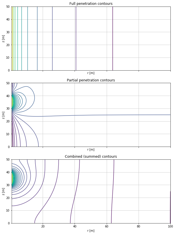
Fig. 7.31 Effect of partial penetration: Top: Head contours due to extraction by a fully penetrating well. Middle: The head change due to partial penetration, (7.8). Bottom: Partial penetration impact superimposed on the heads of the fully penetrating well. (Bottom = Top + Middle). The flow is axially symmetric. \(kD=600\) m\(^{2}\)/d, \(Q=1200\) m\(^{3}\)/d. \(s(r=100)=0\). Drawn are 15 contours between \(s=-1\) and \(s=6\) m. The same contours were drawn in all three pictures.
7.6.3.1. Python implementation of partial penetration
The Python implementation is given in the listing below. The listing also has the code that generated the pictures in Fig. 7.30
def dspp(r=None, z=None, zt=None, zts=None, zbs=None, zb=None, n=20):
    '''Return drawdown effect of partial penetration of well screen without the factor Q/(2 pi kD).
    parameters
    ----------
    r, z : vectors (np.ndarrays)
        vertical and horizontal coordinates
    zt, zts, zbs, zb: four floats
        top aquifer, top screen, bottom screen, bottom aquifer respectively
        The values must decrease to be consistent
    n: int
        maximum in sum
    '''
    if np.any(np.diff(np.array([zt, zts, zbs, zb])) > 0):
        raise ValueError('zt, zts, zbs and zb must be descreasing in value.')
    if np.any(r<=0):
        raise ValueError('r must be all positive')
    if np.any(np.logical_or(z > zt, z < zb)):
        raise ValueError('z must be $\le$ zt and $\ge$ zb')

    D, d = zt - zb, zts - zbs
    R, Z = np.meshgrid(r, z)

    ds = np.zeros_like(R)
    for i in range(1, n + 1):
        p = i * np.pi/D
        ds += (1/i) * (np.sin(p * zts) - np.sin(p * zbs)) * np.cos(p * Z) * K0(p * R)

    return 2 / np.pi * (zt - zb) / (zts - zbs) * ds


# Example worked out
rw = .5 # well radius
R0 = 100. # Fixed head boundary
zt, zts, zbs, zb = 50, 40, 30, 0
r = np.logspace(np.log10(rw), np.log10(R0), 100)
z = np.linspace(zb, zt, 101)
R, Z = np.meshgrid(r, z)

Q = 1200 # m3/d
kD = 600 # m2/d
S = 0.0

s = Q / (2 * np.pi * kD) * np.log(R0 / R)
ds = Q / (2 * np.pi * kD) * dspp(r, z, zt, zts, zbs, zb, n=20)

fig, ax = plt.subplots(3, 1, sharex=True, sharey=True)
fig.set_size_inches(10, 14)
ax = ax.ravel()
titles = ['Full penetration contours', 'Partial penetration contours', 'Combined (summed) contours']
for a, title in zip(ax, titles):
    a.set_title(title)
    a.set_xlabel('r [m]')
    a.set_ylabel('z [m]')
    a.grid()

levels = np.linspace(np.floor(np.min(s + ds)), np.ceil(np.max(s + ds)), 50)
ax[0].contour(r, z, s, levels=levels)
ax[1].contour(r, z, ds, levels=levels)
ax[2].contour(r, z, s + ds, levels=levels)
7.6.4. Questions
What are the properties of the groundwater system leading to a Hantush-type of drawdown in a pumping test? Or: what groundwater system envisioned Hantush when he developed his well formula?
How does the final drawdown expressed in terms of the Hantush-well solution relate to the steady state solution for a well in a semi confined aquifer? Write down your answer mathematically.
At what time does the Hantush drawdown reach half its final steady-state value? Give your answer in mathematical terms.
What is the characteristic time of the adaptation of the head in a semi confined aquifer to a sudden change of the barometer pressure?
Explain why the Hantush type-curves with the lowest \(r/\lambda\) ratio resemble the Theis-type curve most?
Explain why the Theis type curve is an extreme case of the Hantush type curve?
What is the characteristic length \(\lambda\) of a semi-confined aquifer (or, alternatively, the spreading length)? Give your answer mathematically.
How does the Hantush-type curve change when the spreading length is increased?
Explain this change in terms of the transmissivity of the aquifer and the resistance of the overlying aquitard.
What is the general shape of the Hanush-well function graphed using a linear vertical and logarithmic horizontal axis?
Consider an semi-confined aquifer with a constant transmissivity \(kD=900\,\mathrm{m^{2}/d}\) and \(S=0.001\) with the vertical resistance of the overlying layer equal to \(c=400\,\mathrm{d}\). For an observation point at \(r=600\,\mathrm{m}\) distance, determine when the drawdown has become steady state (to at least to 95%). Use the Hantush-type curves to determine your answer.
For the same situation, when is the drawdown at this point equal to half the final drawdown?
For the same situation, when becomes the drawdown essentially larger than zero, say at least 5% of the final drawdown. Tip: use the Hantush type curves to determine your answer.
What is the relation between the the answer to the previous question and the radius of influence of the Theis well?
The head in a building pit of \(50\times50\) m extent, dug into a semi-confined aquifer with transmissivity \(kD=1000\,\mathrm{m^{2}/d}\), resistance \(c=360\,\mathrm{d}\) and storage coefficient \(S=0.002\) has to be lowered by 3.5 m. The wells are placed in the corners of the building pit. How long does one need to pump to reach the steady-state drawdown and what is the final drawdown in the center of the building pit?
What will be the head in the building pit one day after pumping started?
What will be the head in the building pit one day after pumping ended?
What is partial (screen) penetration?
When is partial penetration important? To how far away from the well?
A screen penetrates the first third of the aquifer depth. Explain how the drawdown is affected by the partial penetration relative to the drawdown due to a fully penetrating well? Indicate where the drawdown is more and where it is less than the drawdown due a a fully penetrating screen.
Why is the effect of partial penetration steady already after a short time after the extraction from the well started?
How could you handle partial penetration in a real case when you have to determine the drawdown from a screen that only penetrates part of the aquifer thickness.
7.7. Delayed yield (delayed water-table response)
7.7.1. Introduction
Pumping-tests drawdowns do not always resemble the Theis or Hantush type curves; sometimes the drawdown shows a double dip, which is known as delayed yield. Because delayed yield is quite ubiquitous, it has been studied extensively by scholars in the past, most noticeably by Boulton (1963), Pricket (1971) and Neuman (1974, 1975). While Boulton (1963, 1973) introduced an extra delay parameter to explain the phenomenon, Pricket (1971) demonstrated for a large number of pumping tests in his home state in the USA that the Boulton solution well matched the curves obtained from real-world tests. However, there was no direct physical mechanism behind Boulton’s delay parameter. It remains, therefore, unclear what its precise origin was. It was often assumed that it had to be the unsaturated zone, which is not accounted for in the known groundwater flow solutions. And, indeed, early groundwater-flow models, that accounted for saturated and unsaturated flow simultaneously were able to match the curves that had been measured by Pricket (1971) (see also Cooley and Case (1973)). However, it was Neuman (1974), who solved the problem by showing that the delayed yield could be completely described by the combination of elastic storage, which operates throughout the aquifer, and and storage from the decline of the water table, which is generally accounted for by specific yield. Neuman (1974, 1975) derived an analytical solution for the flow to a well in a water-table aquifer, while taking into account vertical flow components. He showed that the released water initially stems from elastic storage, due to the expansion of the water and the compaction of the soil skeleton, which is a fast process due to the low value of this storage. He further showed that very soon after the start of the pump, the water table starts declining, which releases much more water by emptying pores near the water table, which, therefore is a slow process. It means that after some time, the release of pore water at the water table becomes the dominant process. The result in drawdown line is a graph that resembles two Theis curves, an early Theis curve in accordance with the elastic storage, and a late Theis curve, in accordance with specific-yield storage.
7.7.2. Water-table aquifer
We may show the phenomena on the hand of some numerical simulations as shown in Fig. 7.32. The first picture shows the drawdown versus time for a number of points at different distances from the well and for different depths as expressed in % of the aquifer thickness. The colors correspond to three depths. The blue curves are near the top of the aquifer, the magenta curves in the center of the aquifer, and the green curves near the bottom. As the figure indicates, the drawdowon differs with depth, but only for piezometers that are not far from the well; at later times this difference disappears. The second picture in the same figure shows the depth-averaged drawdown for a number of distances from the well. The later curves correspond to larger differences. One sees that the curves initially correspond to the Theis drawdown computed for the elastic storage coefficient, while later on they match the drawdown that corresponds to the Theis solution for the specific yield. The shorter the distance to the well, the more pronounced the transition between the two Theis curves is. Obviously, the curves that correspond to the larger distances are later. The effect of depth has been eliminated from the second chart by taking the average head over the full depth of the aquifer at each distance. The third picture in Fig. 7.32 demonstrates the difference of the drawdown at different depths at the same location, which was chosen at \(r=28.4\) m from the well. From these graphs, it becomes especially manifest that the closer to the water table, the later the drawdown graph.

Fig. 7.32 Delayed yield in a water table aquifer with a fully penetrating screen. The black lines in all three curves correspond with the Theis drawdown. The middle picture shows the elevation-averaged drawdown at different distances from the well. All lines are blue, but the closer to the water table, the later the drawdown is. The third pictures shows the drawdown at 28.4 m from the well at different depths. The colors indicate the depths, blue is shallow, then black then yellow and finally green for the deepest piezometer. The first figure shows the drawdown at a number of distances and at three different depths. Blue is shallow depth, magenta is the center of the aquifer and green near the bottom of the aquifer.
These graphs in Fig. 7.32 were computed using a numerical axially-symmetric model with elastic storage everywhere, but only specific yield at the water table. There is no unsaturated zone in the model. This is in accordance with Neuman (1972) who explained that the phenomenon of delayed yield can be fully explained by the simultaneous action of the elastic storage in the whole aquifer and the specific yield at the water table.
7.7.3. Generalization to semi-confined aquifers
We may now generalize delayed yield, by extending it to any groundwater system in which a water table will decline in a reaction to pumping. This especially holds true for semi-confined aquifers. The Hanush assumptions underlying his solution include a fixed head in the overlying layer. When in reality this head cannot be maintained, it will cause a delayed-yield effect. This may be the case in many practical situations without it being determined in a pumping test, because the pumping has stopped long before the delayed yield would become visual in the drawdown curves. The reason is the delay that is caused by the resistance against vertical flow from the overlying layer. That this is the case, is explained by the characteristic time for filling the semi-confined aquifer given an initial head difference with the overlying layer. This characteristic time, \(T\), equals \(T=Sc\) where \(S\) is the elastic storage coefficient of the aquifer and \(c\) the resistance of the overlying layer against vertical flow. With typical values of say \(S=0.001\) and \(c=500\) d, we have \(T=0.5\) d. This means that a sudden lowering of the head in the semi-confined aquifer would be fully compensated by increased leakage in about \(5T\approx2.5\) d. This characteristic time affects only the level of the transition zone between the two Theis curves. We can show this by computing the drawdown in a semi-confined aquifer. For this we use an aquifer system consisting of a resistance cover layer that is \(D_{cover}=12\) m thick on top of a \(D_{aquif}=35\) m thick aquifer. The well is fully penetrating. Four models are compared that differ only in the vertical resistance of the cover layer, with values is \(c=[10,100,1000,10000]\) days respectively. Specific yield is \(S_{y}=0.2\), the elastic storage coefficient of the aquifer is \(S=0.002\), i.e. \(S_{s}=S/D_{aquif}\); the hydraulic conductivity of the aquifer is \(k_{h}=10m/d\), hence the transmissivity \(kD=350\,\mathrm{m^{2}/d}\). The results are presented Fig. 7.33.
This figure shows the drawdown averaged over the thickness of the aquifer for different distances from the well. We expect the first branch of the graphs to resemble Hanush’s semi-confined drawdown, for which the value of \(r/\lambda\) determines the elevation of their horizontal equilibrium branch. The spreading lengths of the four models are \(\lambda=[59,\,187,\,,591,\,1870]\) m respectively. The lower the value of \(r/\lambda\), the more the Hantush curve deviates from the Theis curve. This effect is clearly visible when the first picture is compared with the fourth. When the vertical resistance is high, the transfer to the late Theis curve is much delayed. One sees this in the fourth picture, where the graphs don’t even reach the second Theis branch at the end of the simulation time, which was as large as 600 days! When the resistance is low, as in the first figure , the graphs do show a clear transfer from the elastic Theis curve to the water-table Theis curve (first picture). The picture also shows that the drawdown for points near the well resemble the elastic Theis curve, while the points at large distances do not reveal any elastic behavior; they immediately follow the specific-yield Theis curve. The reason is that the first branch should follow Hantush which has an equilibrium \(Q/\left(2\pi kD\right)\mbox{K}_{0}\left(r/\lambda\right)\), which approaches zero for large \(r\). Hence, points at larger \(r\), say at \(r>3\lambda\) will never see the elastic drawdown due to the leakage. The second branch, however, is a pure Theis curve, which has no equilibrium, because it has no recharge (all its water comes from water-table storage). Therefore, points far away from the well will eventually all feel the phreatic drawdown as predicted by Theis (if there are no head boundaries might prevent this).
To determine the resistance of the overlying layer, one should use the piezometers that reach a Hantush-equilibrium and use the Hantush solution to interpret them. This also yields the elastic storage coefficient. If the test is sufficiently long, so that one or more piezometers reach the phreatich Theis branch, then also the specific yield of the overlying layer can be determined by applying the Theis solution to the second branch. As was said earlier, the resistance of the overlying layer does not determine the position of the two bounding Theis curves; it only determines the height of the horizontal branch of the curves where they transfer from the elastic to the specify yield Theis curve.
the more
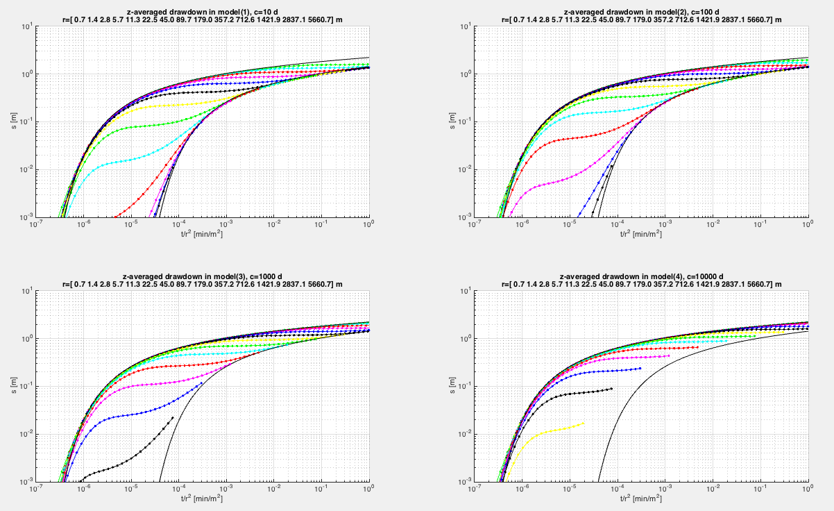
Fig. 7.33 z-averaged drawdown in the aquifer at different distances. Four models differing only in the vertical resistance of the top layer. The Theis elastic storage Theis curve and the specific yield Theis curve are also shown (black lines)
Fig. 7.34 shows the drawdown at one distance, i.e. \(r=28.4\) m, in the top of the overlying layer and in all 35 model layers of the aquifer. First of all, one sees that the head difference between the top and the bottom of the aquifer can be neglected; only the model with the low resistance shows a small difference. This is because in that case the the vertical velocities in the aquifer are large enough to cause a small head loss between the top and the bottom of the aquifer (notice that \(k_{z}=k_{r}=10\,\mathrm{m/d}\) was used). Again, one observes that the horizontal branch climbs with reduced \(r/\lambda\) between the four models. The blue line is the drawdown in the top of the overlying layer, i.e. that of the water table itself. This blue line thus reveals the emptying of the top layer due to the downward leakage invoked by the drawdown in the pumped aquifer below.
7.7.4. The two Theis bounding curves
It was explained before that position of the two bounding Theis curves only depend on their respective storage coefficients and not on the resistance of the covering layer. Notice that we have for the two Theis curves
Hence, the horizontal axes of both Theis curves only differ in their storage coefficient. And so
Hence the horizontal axis of the specific-yield Theis curve is the one of the elastic-storage Theis curve multiplied by \(S_{y}/S\). On the logarithmic scale this is a horizontal shift. Because we have chosen values \(S_{y}/S\)=100, the second Theis curve is shifted over exactly two log-cycles to the right of the first, elastic-storage Theis curve, which can be verified immediately in the graphs.
This also implies the following for the determination of the specific yield from a pumping test that shows a clear delayed-yield behavior. Simply determine the horizontal shift of the second with respect to the first Theis curve, which is factor \(\tau\), and then apply \(S_{y}=\tau S\).

Fig. 7.34 The drawdown at \(r=28.4\) m from the well in the top of the overlying layer and i all 35 model layers of the aquifer for for models differing only in the resistance of the overlying layer. The blue line is the drawdown of the water table, all 35 other lines are at different elevation in the aquifer at the same distance from the well, they essentially fall on top of each other.
Fig. 7.35 shows the drawdown of the water table (blue lines), at the top of the aquifer (color cyan) and at the bottom of the aquifer (magenta) for different distances from the well as noted in the title of the pictures. The figure is essentially equal to the previous picture but the graphs are now drawn for several distances. Once again, the time-drawdown curves for points inside the aquifer stay between the two bounding Theis curves. The curve for the water table lags behind and only joins the specific-yield Theis curve late. This join point falls later the higher the vertical resistance of the overlying layer and the distance from the will. The lower the resistance of the overlying layer, the more will this semi-confined aquifer system resemble the purely phreatic aquifer system that we discussed in the beginning of this chapter.
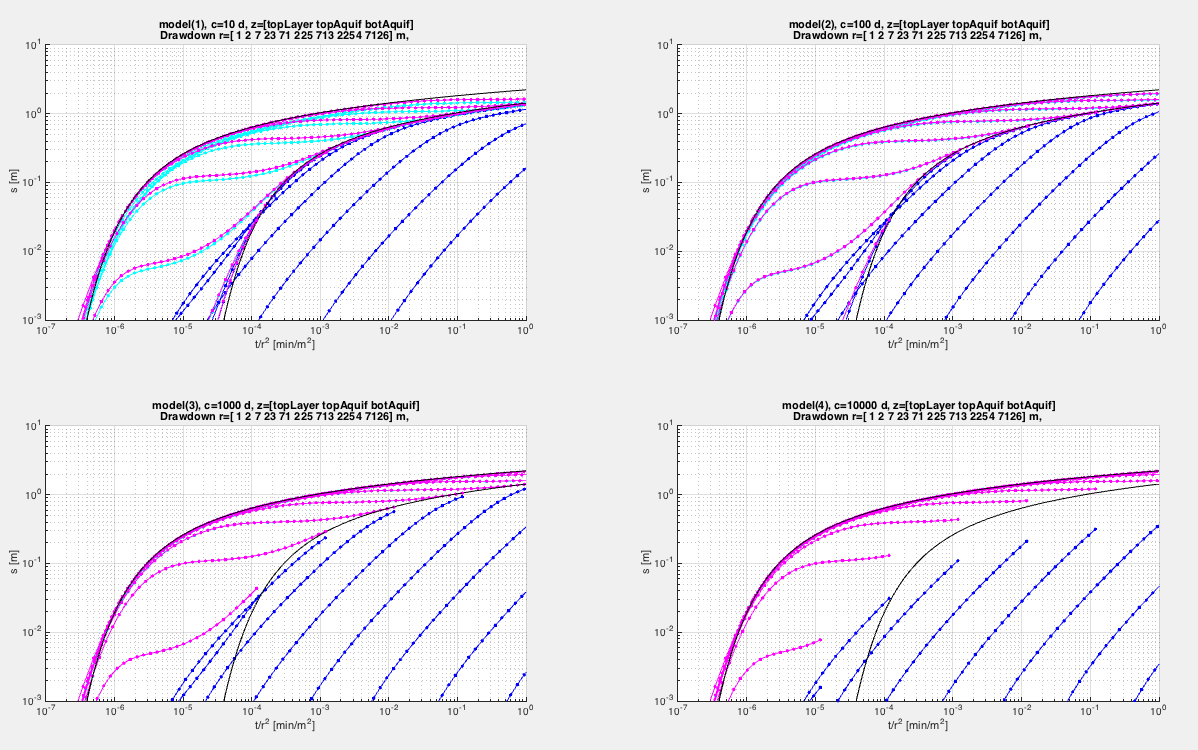
Fig. 7.35 Drawdown in overlying layer (water table, blue), top of the aquifer (cyan) and bottom of the aquifer (magenta) for different distances to the well.
7.7.5. Influence of partial penetration of the well screen
It should be clear that partial penetration causes the drawdown near the well screen to become larger than the Theis drawdown predicts. Hence, one should first correct piezometers closer than about 1D from the well for partial penetration (see section on partial penetration) before analyzing any pumping test. This is illustrated in Fig. 7.36. It shows the drawdown in the top (cyan) and bottom (magenta) of the aquifer for a nearby point ( \(r=9\) m, thick lines) and a distant point ( \(r=90\) m, thin lines). The figure s show that at a point at a large distance from the well is not influenced by partial penetration, as the darwdown in the top and bottom of the aquifer are practically the same and the curves stay between the Theis envelopes, which are the same as in the cases with fully penetrating screens. However, a point close to the well, i.e. less than about 1 to 1.5 aquifer thicknesses away, may experience a serious deviation caused by partial penetration. The point opposite the well screen at the top of the aquifer (thick cyan line) has a drawdown that is larger than that for a fully penetrating screen; the point at the same distance but at the bottom of the aquifer (far below the screen, thick magenta line) has a much lower drawdown than would be the case with a fully penetrating screen. Moreover, these differences do not disappear with time. On the other hand, if we correct for partial penetration by subtracting the effect from all measurements, we regain the fully penetrating drawdowns, which are then directly amenable to interpretation using the standard solutions of Theis and Hantush.
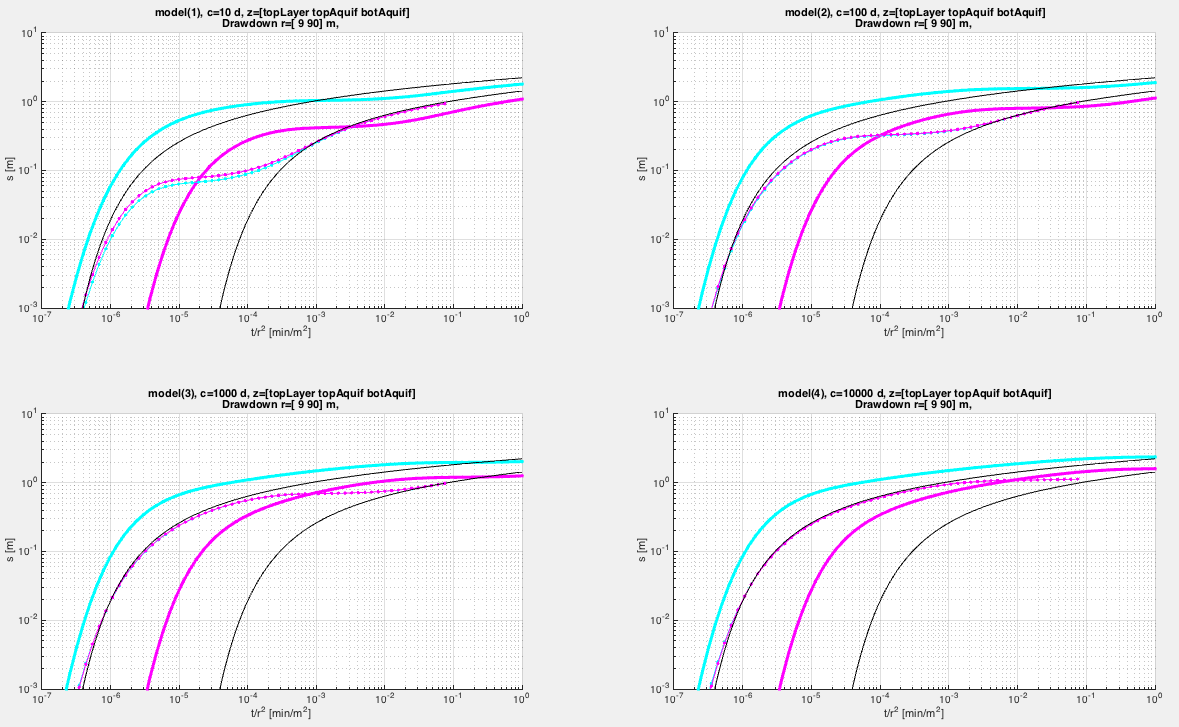
Fig. 7.36 Effect of partial penetration. The screen of only 7 only perforating the top of the 35 m thick aquifer. Drawdown in top and bottom of the aquifer at 9 and 90 m from the well.
7.7.6. Questions
Explain the cause of delayed yield.
Is delayed yield limited to water table aquifers?
What are the bounding curves of the delayed yield curves.
How do the two bounding curves of the delayed yield relate? (What is the relation between the two?)
What determines the elevation of the transition curve (the more or less horizontal branch of the delayed yield curve between the two bounding curves)?
7.8. Large-diameter wells (not for the exam)
The solution of Theis for transient flow in an unbounded confined or unconfined aquifer is based on the assumption that the storage inside the well casing can be neglected. While this is generally a valid assumption for tube wells, and, therefore, for wells in semi-confined and confined aquifers, it may not hold in unconfined aquifers when large-diameter dug wells are used, such as the one shown in figure 44, which is a picture of a large open well in India. Especially when the transmissivity of the aquifer is low, the storage in a large diameter well represents a large portion of the water extracted, at least on the short run, and will thus have a substantial influence on the drawdown. This influence must be taken into account when interpreting drawdown tests on such wells. It should be clear that the formula for a large-diameter well will also hold true when pumping water from a pond.
Papadopoulos and Cooper (1967) (see Kruseman and Ridder (1994), p175) derived an analytical solution for the drawdown in a fully penetrating large-diameter well, taking into account the storage in the casing of the well. The partial differential equation upon which it is based is the same as the one used by Theis. However, the boundary condition at the well face differs; the extraction must now match both the inflow from the aquifer and the drawdown inside the well casing. It thus becomes
where \(Q\) is the constant extraction from the well for \(t>0\). Notice the difference between the well radius \(r_{w}\) and the radius of the well casing \(r_{c}\).

Fig. 7.37 A large-diameter well having a well casing radius \(r_{c}\) different from the well-bore radius \(r_{w}\)
The solution was derived by means of the Laplace Transform, while linearizing by taking \(kh\approx k\overline{h}\). It reads
with
and in which
\(\mbox{J}\left(-\right)\) and \(\mbox{Y}\left(-\right)\) are Bessel functions and \(\alpha=r_{w}^{2}S/r_{c}^{2}\) with \(S\) the storage coefficient (specific yield) and \(u_{w}=\frac{r_{w}^{2}S}{4k\overline{h}t}\).
These expressions may be implemented in Python (see listing below). Type curves for different values of \(\alpha\) but constant ratio \(r_{w}/r_{c}=1\) are given in Fig. 7.38.
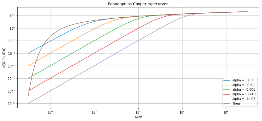
Fig. 7.38 Large-diameter well type curves of Papadoulos-Cooper function \(\mbox{F}(u_{w},\alpha,\frac{r}{r_{w}})\) for different values of a versus \(1/u_{w}\), for \(r=r_{w}\) and \(r_{c}=r_{w}\) and different values of \(\alpha=\left(\frac{r_{w}}{r_{s}}\right)^{2}S\).
def ldwell(rw=None, rc=None, kD=None, S=None, t=None, r=None):
    '''Return the drawdown for a large-diameter well
    parameters
    ----------
    rw, rc: floats
        well radius in aquifer, and wider upper part with storage above the screen
    kD, S: float
        transmissivity and storage coefficient
    t: ndarray
        time at which drawdown is desired
    r: scalar
        distance to well
    '''
    uw = rw ** 2 * S / (4 * kD * t)
    alpha = S * (rw/rc) ** 2
    rrw = r / rw
    return ppco67(uw, alpha, rrw)


def ppco67(uw=None, alpha=None, rrw=None):
    '''Return function values for solution of Papadopulos and Cooper for large diameter well
    parameters
    ----------
    uw : float or array
        uw = rw ** S  / (4 kD t)
    alpha: float
        alpha = S (rw/rc) ** 2
    rrw = r / rw
    '''
    if not np.isscalar(rrw):
        raise ValueError('rrw must be a float (scalar).')
    if not np.isscalar(alpha):
        raise ValueError('alpha must be a float (scalar).')
    if np.isscalar(uw):
        uw = np.array([uw])

    uw = uw[np.newaxis, :]

    beta = np.logspace(-6, 20, 2000)[:, np.newaxis]
    J = beta * J0(beta) - 2 * alpha * J1(beta)
    Y = beta * Y0(beta) - 2 * alpha * Y1(beta)
    F = 8 * alpha / np.pi * (J0(beta * r / rw) * Y - Y0(beta * r / rw) * J) / (beta ** 2 * (Y ** 2 + J ** 2))

    arg = (1 - np.exp(- beta ** 2 /(4 * uw))) * F
    db = np.zeros_like(beta)
    db[:-1, 0] += np.diff(beta[:, 0]) / 2.
    db[1: , 0] += np.diff(beta[:, 0]) / 2.

    return np.sum(arg * db, axis=0)
Figure 6.36 gives an example of the drawdown in a large diameter well and compares it with the Theis drawdown.
![[fig:Example-of-drawdown-largediameter well]Example of drawdown in large-diameter well. :math:`Q=1200` m\ :math:`^{3}`/d. Other parameter are in the figure title.](_images/exampleLargeDiameterWell.png)
Fig. 7.39 [fig:Example-of-drawdown-largediameter well]Example of drawdown in large-diameter well. \(Q=1200\) m\(^{3}\)/d. Other parameter are in the figure title.
8. Convolution
8.1. What convolution is and how it works
Convolution is applied in many branches of science. Because it is so widely and flexibly applicable, it is important to have a thorough understanding of it.
Convolution is a general principle that can be seen as smart superposition, which allows for efficient simulation of linear systems with arbitrary time (or space) varying inputs. In dealing with groundwater it allows interpreting pumping tests with arbitrarily varying extractions (Olsthoorn 2008). It further allows simulation of the groundwater head due to arbitrarily varying river stages as well has groundwater head fluctuations as a function of varying recharge. It is also heavily used in time-series analysis. In mathematical course books, convolution is mostly explained in connection with the Laplace transform, which has some advantages in dealing with it mathematically. However, it is not necessary to understand or apply it. So we do not need this here. In the end convolution boils down to a moving weighted average of the past input data, in which the weight are the response to a unit pulse.
The essential condition for convolution to work is that the response of the system in question due to some physical pulse is unique and proportional to the magnitude of that pulse. A short rain shower is an example of such a pulse due to which the groundwater level will respond by first rising and subsequently declining until the effect of the shower has completely disappeared. The reaction of the system in question to a pulse of unit magnitude is called the impulse response \(\mbox{IR}\left(\tau\right)\). The impulse response depends only on \(\tau\), i.e. the time \(t_{0}\) since the pulse took place, hence \(\tau=t-t_{0}\) (see Fig. 8.1). Notice that the dimension of the pulse (in this case 1 mm of rain for instance) may be completely different from the dimension of the reaction of the system (change of head or change of flow for instance).
We can subdivide any arbitrary time-input into a series of subsequent pulses, for instance, daily rain figure s can be seen as such a continuous input as well as a series of rain pulses. But also a time-varying pumping rate or river stage, can be regarded as a series of hourly or daily pulses. If one imagines an infinite series of unit pulses glued together, say after \(t=t_{0}\), then for \(t>t_{0}\) we have a continuous unit input (a unit input that is an input with the value equal to 1, like 1 mm/d continuous rain). The response of the system to such a continuous unit input after \(t=t_{0}\) is called the step response, \(\mbox{SR}\left(\tau\right)\). In our example this could mean that the well starts pumping at a rate \(Q=1\) at \(t=t_{0}\) and it keeps pumping with this rate forever.
Notice that most analytic solutions of groundwater flow are, in fact, step responses. For instance, the solution for the change of groundwater head or discharge due to a sudden change of the water level of the river, i.e. the expression \(s\left(x,t\right)=A\,\mathtt{erfc}\left(u\right)\mbox{, with }u=\sqrt{x^{2}S/\left(4kDt\right)}\) is such an example. The same is true for the Theis and the Hantush solutions, they too assume a sudden change from zero to a fixed extraction at \(t=0\), which remains forever constant thereafter.
Because the step response can be regarded as the response due to an infinite number of unit pulses for \(t>t_{0}\), it immediately follows that
In practice, we deal with pulses that have a given duration, such as the rainfall during one day. Of course, the rain will vary during the day, but in the end we may not possess data on a shorter time scale than one day, and, therefore, the daily rainfall may be the best and most detailed data that we than obtain in a given case. We will then probably treat these figure s as the average rainfall for each day as the best approximation of the time-varying precipitation. Of course, if one has hourly data, one may use these data as average values for each hour as the best approximation.
So in general, we will have a series of figure s for daily (or hourly, weekly or monthly) precipitation, evapotranspiration, river stage, extraction rate etc.
We then need the so-called block response \(\mbox{BR}\left(\tau,\Delta\tau\right)\). The bock response is the result of a sudden change of an input variable, for instance rain, with a unit magnitude, that is constant during a given time \(\Delta\tau\) and zero thereafter. It’s the result of a unit pulse of fixed duration. The easiest way to compute the block response is by superposition
Which is what we have been doing by our superposition. For instance, with a well in an groundwater system of infinite extent, that fulfills the presumptions underlying the Theis solution, we may write
Based on the previous superposition we can readily compute the required response of the system using the standard groundwater solutions.
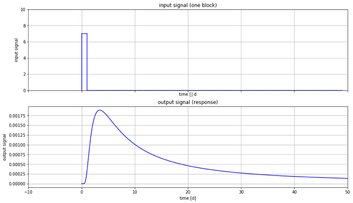
Fig. 8.1 The response of a system to a pulse. Top: the pulse. Bottom: the response of the system to that pulse. Note that the dimensions of pulse and system response are generally different. For example, the discharge as a reaction to a water level change. The response of the system to a pulse holds al the information of the dynamics of the system in question.
Fig. 8.2 shows how standard superposition would work once we have the block response as explained above. For every subsequent actual input pulse of, let’s say a day, we would have multiply the block response and with the actual magnitude of the input to obtain its true response, shown as the set of black curves in Fig. 8.2. Each such system reaction, i.e. each curve, would have to be shifted down the time axis time in accordance with the moment that the pulse occurred, and finally all these reaction curves have to be superimposed to obtain the combined reaction of the system at the desired time. This procedure is what we actually do with superposition and is illustrated in Fig. 8.2.
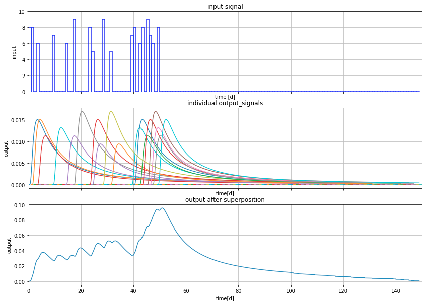
Fig. 8.2 The effect of a series of pulses. Each pulse has its own system response. Top: input signal. Middle: the individual responses, each proportional to the size of its pulse. Bottom: After superposition, i.e. summing all the individual pulses. This is the final output of the system due to the input time series. This is regular superposition in time.
Convolution as a smart way of doing this superposition; it takes a different perspective, one that is illustrated in Fig. 8.3: the essence is that it turns the system response around. Let’s see how that works.
Consider a fixed point in time \(t\), which is a time \(\tau\) after the pulse. The top image shows this pulse, its reaction, the \(\mbox{IR}(\tau)\) or the \(\mbox{BR}\left(\tau,\Delta\tau\right)\). It also shows the considered time \(t\), which is indicated by the vertical line connecting the two graphs. The impact of the pulse at time \(t-\tau\) on the system at time \(t\) is the pulse or block response for \(\tau\) multiplied by the actual height of the pulse, \(p\). Hence the result \(s\) of the pulse is
as indicated in the top figure . Read this formula as the“result of the pulse at t equals the impulse response \(\mbox{IR}\left(\tau\right)\) multiplied by the magnitude of the pulse at time \(t-\tau\), i.e. at \(\tau\) days ago.”
But this is identical with what we get in the bottom figure , where the impulse response is taken relative to \(t\) itself and is reversed in time. Taking this perspective, we would say:“the effect of a pulse at time \(t-\tau\) (or“a time \(\tau\) ago”) equals the reversed impulse response at \(\tau\), i.e. \(\mbox{IR}\left(\tau\right)\) times the height of the pulse at \(t-\tau\).” This is exactly the same as (8.2). This perspective is illustrated in the bottom picture of Fig. 8.3.
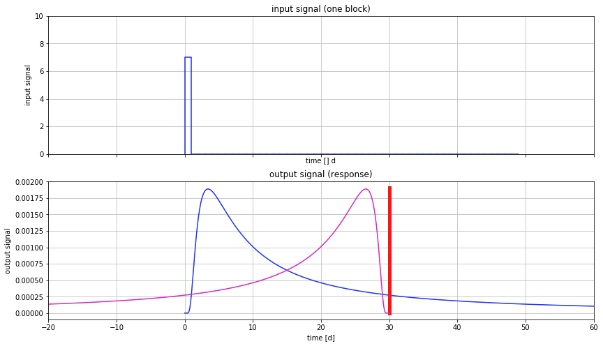
Fig. 8.3 The read bar shows the response of the system 30 days after its pulse. It equals the size of the pulse times the block response. Because the value of the pulse in the top figure is 7, the length of the red bar in the bottom figure , which is the system response, therefore equals 7 times the length of height of the blue block-response. The magenta line is the block-response but inverted in time, so that it looks backward. The distance between the pulse at \(t=0\) and the focus time \(t=30\) is the same for both the original and the reverse block response. Thus, to get the system’s response at \(t=30\) d, just multiply the value of the block-response at the time of the pulse with that pulse.
But this is true the effect at time \(t\) now of any pulse in the past. There is no need to shift the reversed curve at all. So with this perspective, the only thing we have to do to compute the result at time \(t\) due to all inputs of the past, i.e. for time \(-\infty<time<t\), is to multiply each pulse happening a time \(\tau\) ago, that is at time \(t-\tau\) by the value of the impulse response at \(\tau\). This is illustrated in Fig. 8.4, and the result if given in Fig. 8.5. If we compare this procedure with the basic superposition shown in Fig. 8.2, we see that, to compute the state of the system at any given point of time due to what happened in the past, requires only one reversed impulse response, which has to be multiplied with the corresponding the past input (such as rain, river stage or flow rate).
Mathematically this can be generalized as follows
where the input \(p\) is continuous. In the case we split up the past in discrete steps of length \(\Delta\tau\) for which we the average intensity (daily values, say), we use the block response for the corresponding step length \(\Delta\tau\). Then we have
where \(p_{t-\tau_{i}-\Delta\tau\rightarrow t-\tau_{i}}\) means the intensity of the input between \(t-\tau_{i}-\Delta\tau\) and \(t-\tau_{i}\) with \(\mbox{BR}\left(\tau,\Delta\tau\right)\) as defined in (8.1). This procedure is called convolution. It is continuous when we work with the impulse response or discrete in case we work with the block response, what we’ll always do in practice.
Final note: Mathematicians mostly take the integral in (8.3) over \(-\infty<\tau<\infty\), which is equivalent to \(\infty<\tau<0\), because the \(\mbox{IR}\left(\tau\right)\) is zero for \(t<0\) for physical reasons: a response can only exist after it has happened.
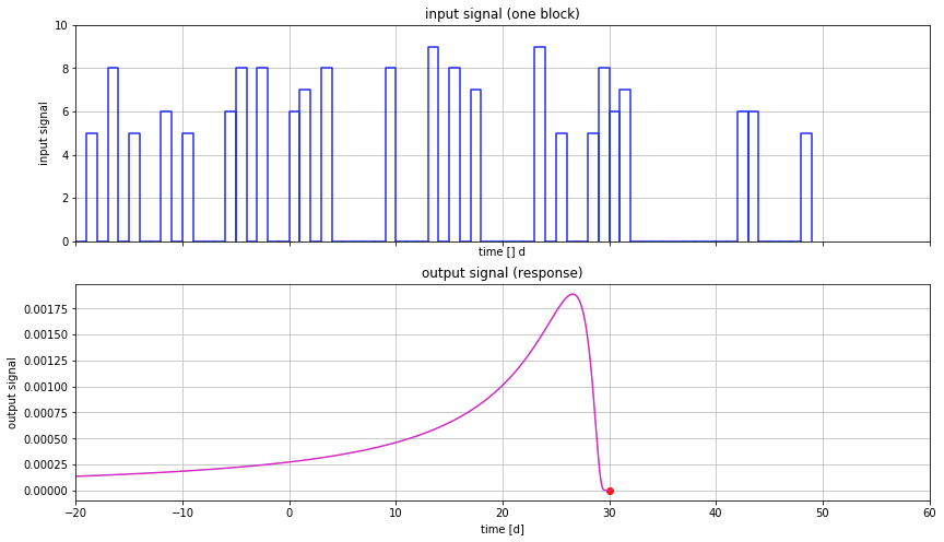
Fig. 8.4 Convolution is the multiplication of the value of the block response \(\mathrm{BR}\left(\tau\right)\), backwards in time from the focus time (here the red dot) multiplied with each corresponding pulse in the past and summing the results to get the system’s response at the focus time, and then shift the focus time, until the whole time axis has been processed. In fact, the system’s response along the time axis is just a moving average of the past input where the weights is the shape of the block-response backward in time.

Fig. 8.5 Result of the convolution.
8.2. Examples
8.2.1. Arbitrarily fluctuating river stage
We can readily carry out a convolution in a spreadsheet or in Python. Python is more straightforward and flexible, therefore we’ll use Python. To do convolution, we need input data, like a time series of the river water level and the impulse response (instantaneous pulse of zero-length but with given magnitude equal to 1) or block response block response (a pulse of of intensity 1 during a fixed time \(\Delta\tau\)), i.e. the river level rises suddenly by 1 m and and falls again by 1 m after time \(\Delta\tau\), which will be the length of our time step. Working with the block response is easiest to comprehend, so we’ll use that. When we have both the input and the block response, we have to carry out the convolution. The convolution for one time t is the past input up to time \(t\), weighted by the block response reversed in time, that is we multiply the input at \(t-\tau\) with the block-response value for \(\tau\). Both the past input and the block response are entire arrays. So, the input array up to time \(t\) is multiplied by the block-response array reversed in time to get the effect of all past input at time \(t\). This is for one point in time, \(t\). To get the result of the convolution for all times, we have to repeat this procedure for all times. What you notice, is, that convolution is in essence a moving weighted average of the input. The input is weighted by the reversed block response and for each time.
In mathematics, convolution is a standard procedure. Many engineering problems are solved through it. Single processing engineers use it all the time to analyze signals. Also in hydrology, convolution is used to analyze time hydrological time series. Therefore, in practice we can make use of standard procedures and functions to carry out the work. In Python, the convolution can be carried out by the function scipy.signal.lfilter, or by the function scipy.signal.convolve.
The first example is to compute the groundwater head resulting from an arbitrary fluctuation of the surface-water level over time of due to an arbitrary varying extraction from a well. The block response is
Let’s use the following figure : \(kD=600\) m\(^{2}\)/d, \(S=0.1\) and we use river level data of the river Meuse at Eijsden on the border between Belgium and The Netherlands. The data can be downloaded from the Internet for a 28 most recent period (Search for “Rijkswaterstaat peil” and find your way). Measurements are taken every 10 minutes. Hence, we use \(\Delta\tau\) is \(10\) min as well. The data for 28 days thus hold 4030 measurements of the river Meuse stage. Reading the .csv file into Python is straightforward using Pandas McKinney (2017). Pandas is the worldwide most-used Python package to handle data tables, a must-know when working with lots of data and tables.
The next listing loads the Pandas module module and dateutil.parser.parse function to parse dates and times. Then it reads the .csv data file for Eijsden specifying the separation between items and which columns to read. Then the data and time columns (both contain just strings) are parsed such that we at a list of datetime objects that is converted into a new index. Finally, we drop the date and time columns we no longer need. The resulting DataFrame than has only one column “Meting” with the measurements, in cm, which we convert to m.
# Get the Meuse water level data for station 'Eijsden'
from dateutil.parser import parse
import pandas as pd

eijs = pd.read_csv('NVT_WATHTE_EIJS.csv', sep=';', usecols=[0, 1, 4])

# Parse the data and time column to get a datetime index
eijs.index = [parse(d + ' ' + t, dayfirst=True) for d, t in zip(eijs['Datum'].values, eijs['Tijd'].values)]
eijs = eijs.drop(columns=['Datum', 'Tijd'])
eijs['Meting'] /= 100. # cm to m
The next 2 lines compute dtau and tau. These lines do that directly from the index, which contains only timestamps (datetime objects). The first line subtracts the second datetime from the first datetime to get the difference as a timedelta object. This is tau already, however to convert it into days as a floating point number, it has to be divided by the datetime object for one day. This generates the value 0.00694. Which is 10 minutes as a day, i.e. 10/(24 * 60). This seems overdone, but the point is, that this method will work for any data set irrespective of the interval length it happens to use.
Subtracting the first datetime from the entire index yields a list of timedelta objects. Dividing this by the timedelta of one day, yields tau in days as a floating point array, with one value every 10 minutes, expressed in days.
dtau = (eijs.index[1] - eijs.index[0]) / np.timedelta64(1, 'D')
tau =np.asarray(eijs.index - eijs.index[0]) / np.timedelta64(1, 'D')
This means that we have now our data in place, as a procedure which automates reading the data and converting them where we need. The job that rests is computing plotting the results for a set of \(x\)-values, with \(x\) the distance of an observation well from the river.
ax2.plot(eijs.index, eijs['Meting'], label='Eijsden')
for x in [25, 50, 100, 200]:
    br = BRriver(tau, dtau, x, kD, S)
    h = eijs['Meting'].mean() +
        lfilter(br, 1.,eijs['Meting'] - eijs['Meting'].mean())
    ax2.plot(eijs.index, h, label='x={:4g} m'.format(x))
    ax3.plot(tau, br, label='x={:4g} m'.format(x))
ax2.legend()
ax3.legend()
The function \(\mathrm{BRriver}\) computes the block response using the following function
def BRriver(tau, dtau, x, kD, S):
    '''Return block response for river level change
    parameters
    ----------
    tau: ndarray
        time after block response
    dtau: float
        width of block that generates the response
    '''
    BR = erfc((x ** 2 * S) / (4 * kD * tau))
    BR[1:] -= BR[:-1]
    return BR
The result is computed using the function scipy.signal.lfilter in this line (shown in the code before):
h = eijs['Meting'].mean() +
    lfilter(br, 1., eijs['Meting'] - eijs['Meting'].mean())
Because we have no infinite past, we start with the mean value of the data that we have a an estimate of the most likely value to start with. Then we apply the linear filter, function lfilter(…) (from the Python module scipy.signal) on the measurements minus the average. We could do without using the average value, but than it takes a run-in period to get rid of the start-value, which is zero by default. The length of the run-in period is equal to the length of the block response. In the current situation, this response is reasonable short, but in other situations that might not be the case, for instance with Theis wells that will never reach equilibrium. We’ll handle a Theis case hereafter.
The results of this exercise are show in Fig. 8.6.
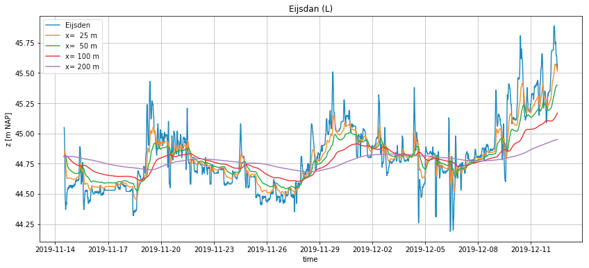
Fig. 8.6 Convolution of river stage. Bottom: the block responses for different distances from the river. Top: The river stage at Eijsden and the resulting fluctuations of the groundwater at different distances from the river. \(kD=600\) m\(^{2}\)/s and \(S=0.2\). The data and simulations are at 10 min interval. Data from Rijkswaterstaat.nl site, The Netherlands.
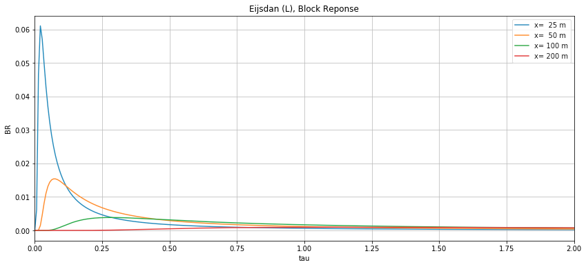
Fig. 8.7 Convolution of river stage. Bottom: the block responses for different distances from the river. Top: The river stage at Eijsden and the resulting fluctuations of the groundwater at different distances from the river. \(kD=600\) m\(^{2}\)/s and \(S=0.2\). The data and simulations are at 10 min interval. Data from Rijkswaterstaat.nl site, The Netherlands.
8.2.2. Impulse response, block response, and step response comparison
Let us now illustrate the difference between impulse response and block response, also for the river stage.
The block response of the river stage is given in (8.5), while the step response is the known solution itself:
The impulse response is obtained by differentiation of the step response with respect to time.
Note that time is embedded in \(u\). For small step widths \(\Delta\tau\), the values of the block response almost equal those of the impulse response when multiplied by \(\Delta\tau\),
This should be obvious because the content of the block response is its intensity, which is equal to \(1\) spread over the duration of the block, which is \(\Delta\tau\), while the impulse response is a pulse of zero duration but of total contents equal to 1. Hence, the numerical value of the block response is \(\Delta\tau\), which is also the value of the impulse response multiplied by \(\Delta\tau\). This is also obvious mathematically,
For values of \(\tau\gg\Delta\tau\) the difference disappears. This is illustrated in Fig. 8.8. The two responses are virtually identical except for smaller \(\tau\) and especially for \(\tau<\Delta\tau\), but this does not affect practical use of either. In practice, I prefer to always use the block response as it is exact and always obtainable from the given step response by a simple subtraction.
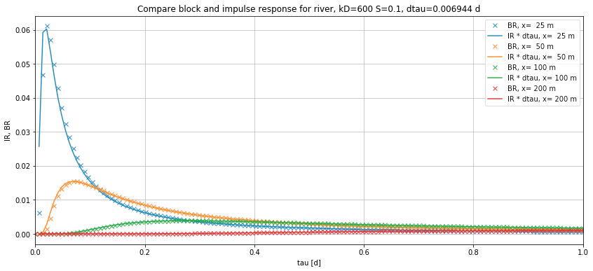
Fig. 8.8 Block response, \(\mbox{BR}\left(\tau,\Delta\tau\right)\), Impulse Response \(\mbox{IR}\left(\tau\right)\times\Delta\tau\) for the situation in Fig. 8.6. One sees that \(\mbox{IR}\left(\tau\right)\times\Delta\tau\) rapidly approaches \(\mbox{BR}\left(\tau,\Delta\tau\right)\) for increasing values of \(\tau\)
8.2.3. Arbitrarily fluctuating extraction of multiple Theis wells
Convolution is also suitable to compute the results of a varying extraction of wells. The same procedure as before can be applied using the Theis (or Hantush) well function.
The block response of the well is
with \(\mbox{W}\left(\dots\right)\) the Theis well function, or function \(\mathrm{scipy.special.exp1}\left(\cdots\right)\), and the notion that the second term only comes in when \(\tau>\Delta\tau\).
def BRtheis(tau, dtau, r, kD, S):
    u = r ** 2 * S /(4 * kD * tau)
    BR = exp1(u)
    BR[1:] -= BR[:-1]
    return BR
For this example the signal can just as well be generated. For this first get a time array. In this case we take days starting in the past, 350 days ago or 350 days before a given date. Then generate an array of random values between 0 and 1. The length of the array is the same as that of the array of times. Subtract 0.5 to get values between -0.5 and 0.5. Filter using a moving average of length 25, to smooth the data somewhat. Finally multiply by Q0 to get a time-varying extraction that covers the entire simulation period.
Q0 = 1200 # m2/d
t = np.arange(-350, 0, 1. ) # past time in days
Qt  = Q0 * (1 + lfilter(np.ones(25)/25., 1., np.random.rand(len(t)) - 0.5))
The generate extraction is shown in Fig. 8.9, top image.
Next the block responses for the well, one for each distance \(r\), have to be computed. The function is given above. The \(\tau\) and \(d\tau\) are readily compute from the time series
dtau = np.diff(t)[0]
tau = np.arange(0, n * dtau, dtau)
The results for the block-responses are show in the second image of Fig. 8.9.
Then the drawdown for the well can be computed for each of the desired distances \(r\). This is done using the block response and the function lfilter(…). It can be computed and immediately plotted
ax2.plot(t, lfilter(br, 1., Qt), label='r = {:4g} m'.format(ri))
The results are shown in the third image of Fig. 8.9. To illustrate its correctness, also the theis drawdown was plotted for the average extraction, i.e. \(Q_{0}\).
A similar plot can be made by plotting the drawdown on logarithmic time axis. However, for that we need to prevent negative times on the time axis, and so we must use the time \(t-t_{0}\), with \(t_{0}\) the time that the well started, which is assumed at the first value of the time series.
ax3.plot(t - t[0], lfilter(br, 1., Qt), label='r = {:4g} m'.format(ri))
The results are shown in the bottom image of Fig. 8.9. Here too, the results of the Theis drawdown or the average extraction are shown on this figure .
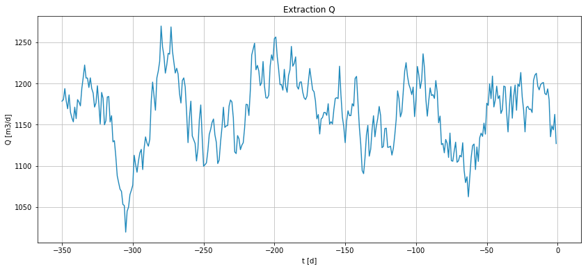
Fig. 8.9 Results of the explained example. Five wells, their discharge (left picture) their drawdown (right picture) and the total drawdown (black line in right-hand picture).

Fig. 8.10 Results of the explained example. Five wells, their discharge (left picture) their drawdown (right picture) and the total drawdown (black line in right-hand picture).

Fig. 8.11 Results of the explained example. Five wells, their discharge (left picture) their drawdown (right picture) and the total drawdown (black line in right-hand picture).
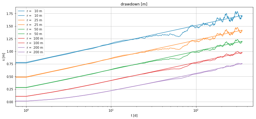
Fig. 8.12 Results of the explained example. Five wells, their discharge (left picture) their drawdown (right picture) and the total drawdown (black line in right-hand picture).
8.2.4. Convolution using recharge as input time series to simulate varying groundwater levels
The solution for drainage after a sudden uniform recharge on a strip of land between two canals with maintained water level was given in chapter [sec:Symmetrical-drainage-from-charcteristic-time] (6.13) . That solution can be seen as en impulse response by itself. When regarding the sudden rise \(A\) as due to a (recharge) shower \(p\), then \(A=\frac{p}{S}\) and we can write that formula, taking \(p=1\) as
The block response can then be approached by
This block response can be code as follows
def IRbasin(tau, x=None, b=None, kD=None, S=None):
    T = b ** 2 * S / kD
    s = np.zeros_like(tau)
    for j in range(1, 20):
        j2p = (2 * j - 1) * (np.pi / 2)
        s += (-1) ** (j - 1) / (2 * j - 1) * np.cos(j2p * x / b) * np.exp(- j2p ** 2 * tau / T)
    return s * 4 / (np.pi * S)
To give an example the following aquifer and width values are used
kD = 600 # m2/d
S = 0.2
b = 200 # m  we'll also use values 750 and 2000 m
x = b * np.array([0, 0.5, 0.8, 0.9, 0.95, 0.98, 0.99])
T = b ** 2 * S / kD # [d] characteristic time
The recharge data are read from the file PT-00-08.txt using module Pandas. We use the index to get the step size \(d\tau\) as the time difference between the first to datestamp objects of the index of the data PE. To take tau sufficiently long we’ll use 7 times the characteristic time. The value of this time, T, is shown in the title of the pictures in Fig. 8.13.
PE = pd.read_csv('PE-00-08.txt', index_col=0, parse_dates=True, dayfirst=True)
PE /= 1000. # convert all to mm/d

dtau = (PE.index[1] - PE.index[0]) / np.timedelta64(1, 'D')
tau = np.arange(0, 7 * T, dtau)
The convolution to compute the head is done using the function lfilter(…) as before, where the recharge is the difference of the column ‘P‘ and column ‘E‘ in the Pandas DataFrame PE.
lfilter(BR, 1, PE['P'] - PE['E'])
Implemented in a loop, so that is the head can be computed for number of \(x\)-values. Note that \(x\) is the distance to the center of the basins. The \(x\)-values use are computes as a fraction of the half-width \(b\).
x = b * np.array([0, 0.5, 0.8, 0.9, 0.95, 0.98, 0.99])
Then the loop that computes the head and plots the head for each \(x\) on a single figure .
title=  '2b = {:4g} m, kD = {:4g} m2/d, S = {:4g}, T = {:.0f} d'.format(2 * b, kD, S, T)
ax0 = newfig(title='Simulation groundwater in basin\n' + title, xlabel='time', ylabel='head')
ax1 = newfig(title='Recharge', xlabel='time', ylabel='mm')

for xi in x:
    BR = dtau * IRbasin(tau, x=xi, b=b, kD=kD, S=S)
    ax0.plot(PE.index, lfilter(BR, 1, PE['P'] - PE['E']), label='x = {} m'.format(xi))
    ax1.plot(PE.index, PE['P'] - PE['E'])
ax0.legend()
Fig. 8.13 gives the results for 3 widths of basin (the width is \(2b\)). It is very clear that the wider the basin, the larger the memory of the system, which is characterized by the characteristic time. This time increase from \(T=13\) d for \(2b=400\) m in the top image to \(T=1300\) d for \(2b=4000\) m in the third picture. The factor \(100\) is due to the fact that the characteristic time is proportional to the square of the basin width. The block responses for the three basins that differ only in width are given in Fig. 8.17. The large the memory of the groundwater system, the longer the past period over which the recharge is integrated and has an effect on on the head. Because the average recharge in this example (Dutch data) is positive, a large system must show heads that are always above its boundaries (zero). This is indeed the case in the third picture, and more so for points farther away from the boundaries, i.e. more to the center line of the basin. The shorter the system memory, the more often a dry period can cause the heads to fall below the water levels of bounding canals or rivers. Also, the shorter the memory the lower will the average head be relative to the bounding surface water level. This simulation is realistic, except for the fact that it was assumed that the water from a recharge pulse reaches the groundwater immediately. While this may be a good approximation for shallow groundwater, it is not realistic where the water table is 10 m or more below ground surface. In such situations, it may take several months before a recharge pulse causes the flow from the unsaturated zone into the saturated zone to increase. A thick unsaturated zone causes the recharge arrival in the saturated zone to be delayed and somewhat smoothed. If this delay and smoothing can be estimated from an unsaturated zone analyses of from measurements, it may be included by filtering the recharge time series before using it has input for the head simulation. Filtering is just a moving averaging procedure, hence a convolution, which can be carried out with the same function lfilter(…), all we need is a block response that relates the recharge to the flux at the bottom of the unsaturated zone.

Fig. 8.13 Simulation by convolution of head in river basin driven by varying recharge.
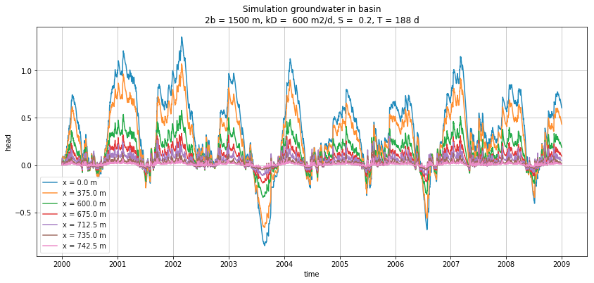
Fig. 8.14 Simulation by convolution of head in river basin driven by varying recharge.
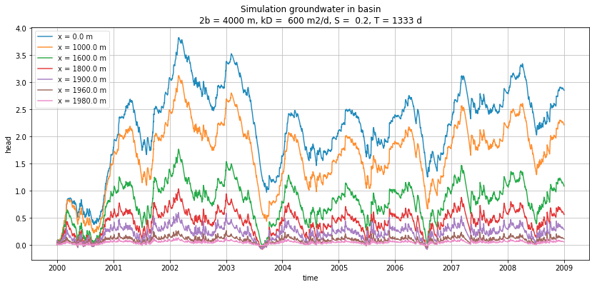
Fig. 8.15 Simulation by convolution of head in river basin driven by varying recharge.
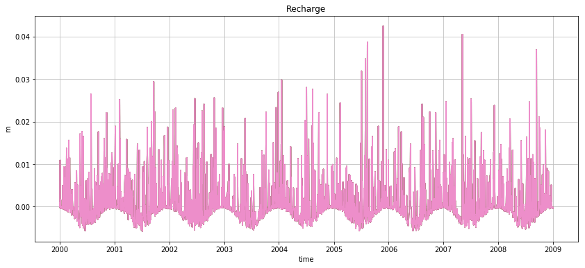
Fig. 8.16 Simulation by convolution of head in river basin driven by varying recharge.
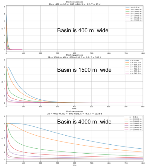
Fig. 8.17 Block responses ( \(d\tau=1\) d) of the head after a 1d long recharge pulse for the 3 basins in Fig. 8.13 that only differ in width. The different curves for each basins represent distance from the center of the basin. The positions relative to the width of each basin are the same in the three figure s, namely 0%, 50%, 80%, 90%, 95%, 98% and 0.99% of the half width of the basin measured from the center.
8.3. Questions
Explain what convolution is and how it compares with superposition.
Explain impulse response, block response and step response.
Why did we reverse the direction of the time series in the implementation of convolution in the spreadsheet.
What is the consequence of the lack of past data on the results of convolution, especially on those of the oldest times, for which there are no past data available?
In terms of system responses, what, in fact, are the solutions of groundwater flow like those for a sudden change of river stage and the Theis and Hantush well functions?
Explain in your own words the meaning of (8.3)?
How does the impulse response relate to the step response mathematically?
How can you compute the block response \(\mathrm{BR}\left(\tau,\Delta\tau\right)\) of a system?
9. Laplace solutions (illustration, not for exam)
9.1. Sudden head rise at the boundary of a one-dimensional semi-infinite aquifer
The Laplace transform is used to solve the one-dimensional partial differential equation, known as the diffusion equation. The Laplace transform removes time from the partial differential equation after which we only have to solve a steady state situation, whose solution we already know. Once we have this solution in Laplace space we convert it back to time by looking up the result in a Laplace transform table (Abramowitz and Stegun (1972)).
We consider a one-dimensional aquifer with constant transmissivity \(kD\) with initial head zero at a bounding a river at \(x=0\) whose water level is suddenly increased at \(t=0\).
The differential equation is
with as boundary conditions:
Taking the Laplace transform of the differential equation and its boundary conditions yields:
The solution in Laplace space is easily found as it is the same as the stationary solution for a 1-D leaky aquifer with fixed head at \(x=0\):
The steady state solution was for the differential equation
From which it follows that
So that
The inverse transform is given by Abramowitz and Stegun (1964, p1026, item 29.3.83):
Hence, with \(\kappa\) replaced by \(\frac{x^{2}S}{kD}\) we find
Which is the sought solution.
9.2. Laplace solution for the Theis well function
The Laplace transform is one method, perhaps the most practical and universal to solve partial differential equation that depend on time. The Laplace transform removes the time derivative from the partial differential equation (Bruggeman 1999), after which is can be solved as a steady-state problem. Once we have the steady-state solution in Laplace space, we have to transfer it back to time, which is done with conversion tables, see Abramowitz and Stegun (1972).Bruggeman (1999) gives a full derivation for the leaky aquifer case of Hantush. Here we apply the Laplace transform on the transient well extraction studied by Theis. You may also want to look at a paper on this, Loáciga (2009), showing various approaches.
The partial differential equation for transient flow in an aquifer with constant transmissivity is
Denoting the Laplace transform of \(\overline{\phi}=L\left\{ \phi\right\}\) and the inverse transformation by \(\phi=L^{-1}\left\{ \overline{\phi}\right\}\), the Laplace transform of \(\ref{eq:pdf-aximetric-theis}\) through [eq:BC3-aximetric-theis], becomes, with \(p\) as the Laplace constant:
Its general solution we already know from steady state groundwater flow:
It is clear that \(B\) must be zero to meet the condition for \(r\rightarrow\infty\), because \(I_{0}\left(\infty\right)=\infty\).
The flow at \(Q_{r}\) distance \(r\) becomes in Laplace, where \(Q_{r}/\left(2\pi kD\right)\) is a time-invariant, becomes
so that, after substituting \(B=0\) and \(A\) from the previous expression ((9.8)) into (9.6) yields
Because \(raK_{1}\left(ra\right)=1\) for \(r>0\) and \(a\) a positive constant, we have, writing \(Q_{r}\rightarrow Q_{0}\)
because
with, in our case,
and from the tables of the Laplace transforms (Abramowitz and Stegun (1972), p1028)
we find
Replace
Where \(\mathrm{E}_{1}\left(-\right)\) is the exponential integral, a standard function in Matlab and tabled in many groundwater hydrology books as the Theis well function \(\mathrm{W}\left(u\right)\). It can be developed in a series expansion as well (Abramowitz and Stegun (1972), p228-229):
9.3. Stehfest for numerical back-transformation of Laplace solutions
This can be used to numerically back-transform the results from Laplace space to normal time. Still some work to do to work this out.
10. Bibliography
Abramowitz, M, and I A Stegun. 1972. Handbook of Mathematical Functions with Formulas, Graphs, and Mathematical Tables. Edited by M Ambramowitz and I A Stegun. Wiley.
Bear, Jacob. 1988. Dynamics of Fluids in Porous Media. Dover.
Boemen, P J T M, C Lekkerkerker, and W H van der Molen. 1989. “Aardgetijden in Grondwater: Een Voorbeeld Uit Burkina Faso (Earth Tides in Groundwater, an Example from Burkina Faso).” H2o 22 (17): 536–38.
Boulton, N S. 1963. “Analysis of Data from Non-Equilibrium Pumping Tests Allowing for Delayed Yield from Storage.” Proc. Inst. Civ. Eng., November, 469–82.
———. 1973. “The Influence of Delayed Drainage on Data from Pumping Tests.” Journal of Hydrology 19: 157–69.
Bredehoeft, J D. 1967. “Response of Well-Aquifer Systems to Earth Tides.” Journal of Geophysical Research, Earth Surface 75 (12): 3075-30870-19-853368-3.
Bruggeman, G A. 1999. Analytical Solutions of Geohydrological Problems (Developments in Water Science). Elsevier Science.
Carslaw, H S, and J C Jaeger. 1986. Conduction of Heat in Solids. Clarendon Press.
Cooley, R L, and C M Case. 1973. “An Effect of a Watertable Aquitard on Drawdown in an Underlying Pumped Aquifer.” Water Resources Research 9 (2): 434-44790-6743-654-2.
Dufour, F C. 2000. Groundwater in the Netherlands, Facts and Figures. Netherlands. Delft, The Netherlands: Netherlands Insttute for Applied Sciences TNO.
Gun, J A M van der. 1980. “Schatting van de Elastische Bergingscoëfficiënt van Zandige Watervoerende Pakketten (Estimation of the Elastic Storage Coefficient of Sandy Aquifers, in Dutch.” Dienst Grondwaterverkenning TNO, Jaarverslag 1979. Dienst Grondwaterverkenning TNO, Delft, pp 51-61.
Hantush, M S. 1955. “Non-Steady Radial Flow in an Infinite Leaky Aquifer.” Transm. Amer. Geophys. Union 36: 95–101.
Hemker, C J. 1984. “Steady Flow to Leaky Multiple-Aquifer Systems.” Journal of Hydrology 22 (2-3): 355–75.
———. 1985. “Transient Flow to Leaky Multiple-Aquifer Systems.” Journal of Hydrology 81 (1-2): 111–21.
Hemker, C J, and C Maas. 1987. “Unsteady Flow to Wells in Layered and Fissured Aquifer Systems.” Journal of Hydrology 90: 231–49.
Huisman, L. 1972. Groundwater Recovery. MacMillan.
Kamp, G van der, and J E Gale. 1983. “Theory of Earth Tide and Barometric Effects in Porous Formations with Compressible Grains.” Water Resources Research 19 (2): 538–44.
Kruseman, G P, and N A de Ridder. 1970. Analysis of Pumping Test Data. 1st ed. Bulletin 11. Wageningen, Netherlands: ILRI.
———. 1994. Nalysis of Pumping Test Data. Second Edition. Publication 47. Wageningen, Netherlands: ILRI, Wageningen.
Loáciga, H. 2009. “Derivation Approaches for the Theis (1935) Equation.” Groundwater.
Maas, C. 1986. “The Use of Matrix Differential Calculus in Problems of Multiple Aquifer Flow.” Journal of Hydrology 88: 43–67.
McKinney, W. 2017. Python for Data Analysis, 2nd Edition. Beijing etc.: O’Reilly.
Neuman, S P. 1974. “Effect of Partial Penetration on Flow in Unconfined Aquifers Considering Delayed Gravity Response.” Water Resources Research 10: 303–12.
———. 1975. “Analysis of Pumping Test Data from Anisotropic Unconfined Aquifers Considering Delayed Gravity Response.” Water Resources Research 11 (2): 329–42.
Olsthoorn, T N. 2008. “De a Bit More with Convolution.” Groundwater 46 (1): 13–22.
Papadopoulos, I S, and H H Cooper. 1967. “Papadopulos and Cooper Solution for Nonleaky Confined Aquifers.” Water Resources Research 3: 241–44.
Powell, Owen, and Rod Fensham. 2015. “The History and Fate of the Nubian Sandstone Aquifer Springs in the Oasis Depressions of the Western Desert, Egypt.” Hydrogeology Journal 24 (2): 395–406. https://doi.org/10.1007/s10040-015-1335-1.
Pricket, T A. 1971. “Type-Curve Solution to Aquifer Tests Under Water-Table Conditions.” Technical Division NWWA (National Water Well Association Inc., 14.
Rasmussen, T C, and L A Crawford. 1997. “Identifying and Removing Barometric Pressure Effects in Confined and Unconfined Aquifers.” Groundwater 35 (3): 502–11.
Theis, C V. 1935. “The Relation Between the Lowering of the Piezometric Surface and Rate and Duration of Discharge of a Well Using Groundwater Storage.” Transactions of the American Geophysical Union 16: 519–24.
Todd, D K. 1959. Groundwater Hydrolog. John Wiley & Sons Inc.
Todd, D K, and L W Mays. 2005. Groundwater Hydrology. Wiley.
Verruijt, A. 1999. Grondmechanica (Soil Mechanics). Delft, Netherlands: Delft University Press.
Voss, C, and S Soiman. 2014. “The Transboundary Non-Renewable Nubian Aquifer System of Chad, Egypt, Libya and Sudan: Classical Ground- Water Questions and Parsimonious Hydrogeologic Analysis and Modelin.” Hydrogeoly Journal 22: 441–68.
Vries, J J de. 1984. “Holocene Depletion and Active Recharge of the Kalahari Groundwater - a Review and an Indicative Model.” Journal of Hydrology.
Wösten, J H M, G H Veerman, and J Stolte. 1994. Water Retention and Hydraulic Conductivity Functions of Top- and Subsoils in the Netherlands. Wageningen: Wageningen University.